from lec_utils import *

Lecture 2

Python and Jupyter Notebooks

EECS 398-003: Practical Data Science, Fall 2024

practicaldsc.org • github.com/practicaldsc/fa24

Announcements 📣

• The Welcome Survey is due on Monday, September 2nd.
  EECS 370 has the same midterm time as us. If you're in 370, sign up to take their alternate midterm exam the following day.
• Homework 1 will be released tomorrow and will be due on Thursday, September 5th.
• We released a Setup Walkthrough Video to supplement the steps in the ⚙️ Environment Setup page of the course website. Make sure to set up your environment ASAP!
• We also released an "Example Homework" assignment, which you should work through.
  This isn't due, but exists to make sure that your environment is set up correctly, and that you know how to access, work on, and submit homeworks.
• Come to Discussion 1 tomorrow to hear some Jupyter Notebook tips and get started on Homework 1.
  Attend either section, but if space fills up, priority is given to the students who are officially enrolled.
• The course just expanded to 160, so you should be let off the waitlist if you were on it.
• Check out the new Resources tab on the course website, with links to lots of supplementary resources and past exams from similar classes!
• Have any feedback on the course? Let us know at the Anonymous Feedback Form.

Agenda

• The anatomy of Jupyter Notebooks.
• Python.
  Especially, in relation to C++.
• numpy arrays.

We're going to cover a lot quickly. The Textbooks section of the Resources tab on the course website has links to lots of great online resources about this material if you'd like other perspectives.

Question 🤔 (Answer at practicaldsc.org/q)

Remember that you can always ask questions anonymously at this site during lecture!

Have you followed the instructions in the ⚙️ Environment Setup page and set up your environment?

• A. Yes, and I even tested out the Example Homework released yesterday.
• B. Yes, I set up my environment, but haven't run any code yet.
• C. I tried to, but I ran into some errors or got stuck.
• D. I looked at the instructions, but haven't followed them yet.
• E. Haven't started.

The anatomy of Jupyter Notebooks

---

Let's start by familiarizing ourselves with our programming environment.

Jupyter Notebooks 📓

• Often, but not in this class, code is written in a text editor and then run in a command-line interface, or both steps are done in an IDE.

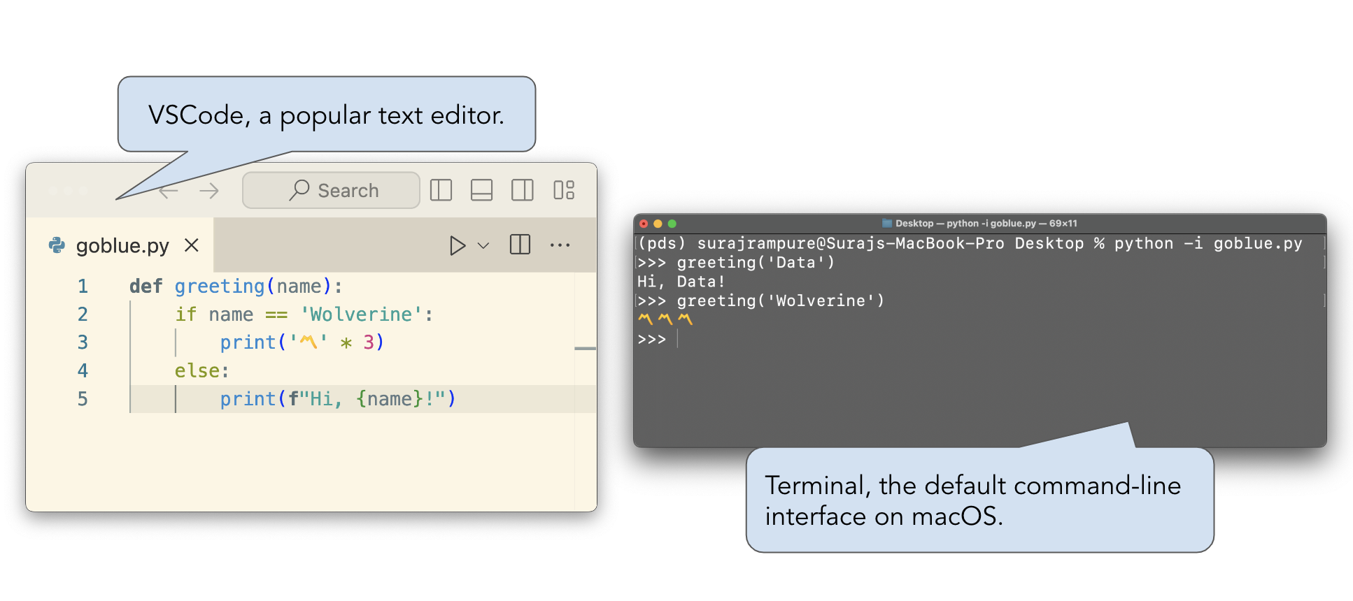
• Jupyter Notebooks allow us to write and run code within a single document. They also allow us to embed text and images and look at visualizations.

Why Jupyter? It stands for Julia, Python, and R, the three original languages they were designed to support.

• .ipynb is the extension for Jupyter Notebook files. .ipynb files can be opened and run in a few related applications, including JupyterLab, Jupyter Notebook, Jupyter Notebook Classic, and VSCode.

The ⚙️ Environment Setup page walks you through how to launch each one.
Note that these lecture slides are a Jupyter Notebook also, we're just using a package to make them look like a presentation.

Cells

The cell is the basic building block of a Jupyter Notebook. There are two main types of cells:

• Code cells, where you write and execute code.
  • When run, code cells display the value of the last evaluated expression.

• Markdown cells, where you write text and images that aren't Python code.
  • Markdown cells are always "run", except when you're editing them.
  • Double-click this cell and see what happens!
  • Read more about Markdown here.

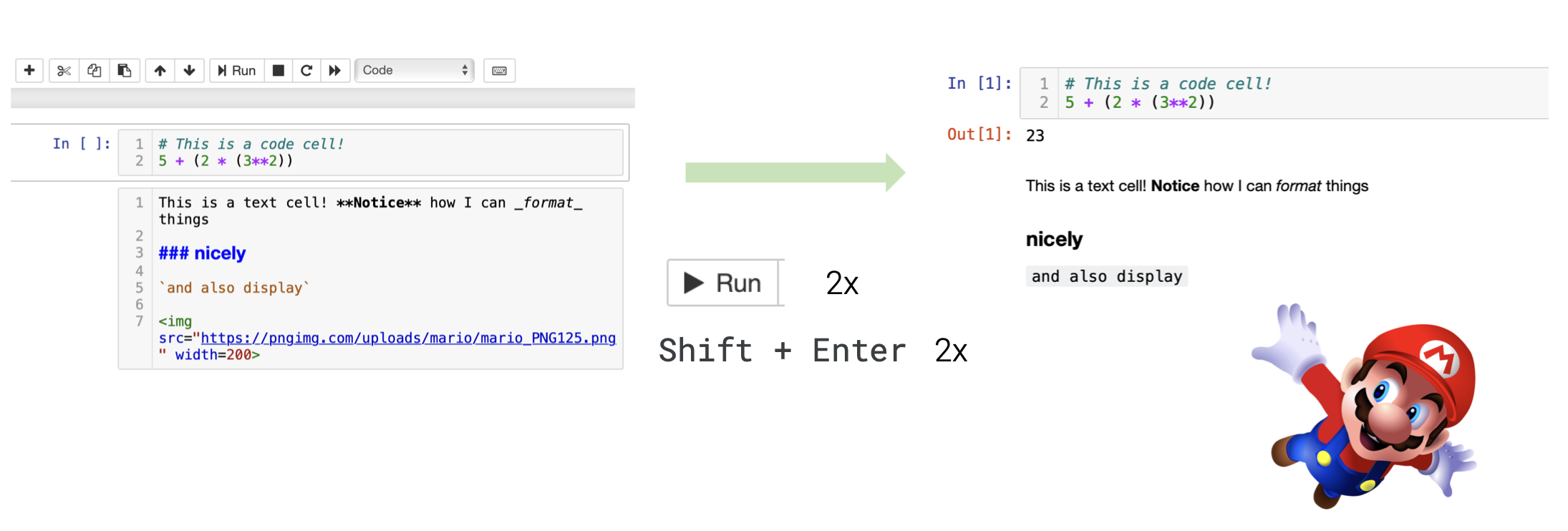A code cell and Markdown cell, before and after being "run".

Using Python as a calculator

To familarize ourselves with the notebook environment, let's run a few code cells involving arithmetic expressions.

To run a code cell, either:

• Hit shift + enter (or shift + return) on your keyboard (strongly preferred), or
• Press the "▶ Run" button in the toolbar.

# When you run this cell, the value of the expression appears, but isn't saved anywhere!
# These are comments, by the way.
17 ** 2

289

# Integer division.
25 // 4

6

min(-5.7, 1, 3) + max(4, 9, 7)

3.3

# Why do we only see one line of output?
2 - 4
18 + 15.0

33.0

# Strings can be created using single, double, or triple quotes.
# There's no difference between a string and a char.
'678' + "9" * 3

'678999'

'''November 26,
''' + "1998"

'November 26,\n1998'

# Put ? after the name of a function to see its documentation inline.
# All notebook interfaces support tab for autocompletion, too.
round?

Signature: round(number, ndigits=None)
Docstring:
Round a number to a given precision in decimal digits.

The return value is an integer if ndigits is omitted or None.  Otherwise
the return value has the same type as the number.  ndigits may be negative.
Type:      builtin_function_or_method

Edit mode vs. command mode

When working in Jupyter Notebooks, we use keyboard shortcuts often. But the keyboard shortcuts that apply depend on the mode that we're in.

Edit mode: when you're actively typing in a cell.

Command mode: when you're not actively typing in a cell.

Hit escape to switch from edit to command, and enter to switch from command to edit.

Keyboard shortcuts

A few important keyboard shortcuts are listed below. Don't feel the need to memorize them all!

• You can see them by hitting H while in command mode.
• You can also just use the toolbar directly, rather than using a shortcut.

Action	Mode	Keyboard shortcut
Run cell + jump to next cell	Either (puts you in edit mode)	SHIFT + ENTER
Save the notebook	Either	CTRL/CMD + S
Create new cell above/below	Command	A/B
Convert cell to Markdown	Command	M
Convert cell to code	Command	Y

Python

---

Let's highlight some key features of Python, and contrast them to C++, a language you've likely used before in EECS 280/281 (though if you've received an override, never taken an EECS class, but have programmed before in another language, you'll be able to follow along, too).

Variable types and code compilation

• In C++, variable types need to be explicitly declared ahead of time, and are fixed (static) once declared. The compiler verifies that all types are consistent before the code is actually executed.

// Compiler error!
            int count = 7 + 9;
            count = "data science";

                    main.cpp:16:9: error: invalid conversion from ‘const char*’ to ‘int’ [-fpermissive]

• In Python, variable types don't need to be declared, and are free to change (dynamic).

Also, note that you don't need semicolons!

# Works just fine.
count = 7 + 9
count = "data science"
count

'data science'

type(count) # The type function returns the type of an object.

str

• Since Python is interpreted, not compiled, it doesn't have any compiler errors. All errors occur at runtime.
  This means that you can "run" lots of buggy code, but you may only spot the issues later on – be careful!

# This function takes in a single argument and returns that argument + 1 / 0.
# Python doesn't stop us from defining the function.
def f(x):
    return x + 1 / 0

f(15)

---------------------------------------------------------------------------
ZeroDivisionError                         Traceback (most recent call last)
Cell In[12], line 1
----> 1 f(15)

Cell In[11], line 4, in f(x)
      3 def f(x):
----> 4     return x + 1 / 0

ZeroDivisionError: division by zero

Variable types and compilers

	Python	C++
Do I need to define the type of a variable beforehand?	No Python is dynamically typed.	Yes C++ is statically typed.
Do I compile my code before running it?	No Python is interpreted; Python code is converted to bytecode line-by-line at runtime. In fact, the standard implementation of Python is written in C (called CPython).	Yes The entirety of a C++ program needs to be compiled to bytecode before it's run. This is part of why C++ is much faster than Python.

• You can use type "hints" in Python, but they aren't verified at runtime.

name: str = 'Junior'
name = 3.14

Jupyter memory model

• Python may be new to you, but in addition, code in a Jupyter Notebook behaves a little differently than code in a text editor + Terminal setup.

• Pretend your notebook has a brain 🧠.

• Everytime you run a cell with an assignment statement, it remembers that name-value binding.

• It will remember all name-value bindings as long as the current session is open, no matter how many cells you create or delete.

# We defined this a while ago, but it still remembers.
# This is a common pattern: writing the name of a variable in a cell of its own
# to check its value.
count

'data science'

• But, quitting your Terminal ends your Jupyter Notebook session, and your notebook will forget everything it knows – you’ll need to re-run all of your cells the next time you open it.

• With this in mind, you should aim to structure your code in a reproducible manner – so that others can trace your steps. Let's look at some practices you should avoid ❌.
  And by others, we mostly mean you, when you come back to your homework the next day.

1. Don't delete cells that contain assignment statements.

# To illustrate the issue, run this cell and then delete it.
age = 23

# If the above cell has been run, this cell will run just fine, even if you 
# delete the cell above. However, once your notebook "forgets" all of 
# the variables it knows about, this cell will error, 
# since `age` won't be defined anywhere!
age + 15

38

2. Don't use a variable in a cell above where it is defined.

# If you run the cell below first, then this cell will run just fine.
# However, once your notebook "forgets" all of the variables
# it knows about, and you run all of its cells in order,
# this will cause an error, because you are trying to use
# `weather` before its defined!
weather - 4

68

# To illustrate the issue, run this cell FIRST, then the cell above.
weather = 72

3. Don't overwrite built-in names!

min(2, 3)

2

min = 17

min(2, 3)

---------------------------------------------------------------------------
TypeError                                 Traceback (most recent call last)
Cell In[31], line 1
----> 1 min(2, 3)

TypeError: 'int' object is not callable

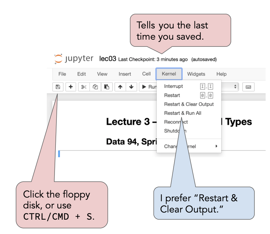
Restarting the kernel

If something doesn't seem right, you can force your notebook to forget everything it currently is remembering and give it a "fresh start". To do so:

1. Save your notebook (by clicking the floppy disk icon or CTRL/CMD + S).

2. Restart your kernel.

The kernel is like the engine of a Jupyter Notebook. We're working with a Python kernel that has our pds conda environment installed.
There exist Jupyter kernels for many languages, including C++!

Aside: Terminal commands in Jupyter Notebooks

You can run command-line operations in Jupyter Notebook cells by placing ! before them.

!ls imgs

broadcasting.jpg         elementwise.jpg          restart-kernel.png
commandmode.png          mdcell.png               text-editor-terminal.png
editmode.png             numpy.png

This can be useful in figuring out the location of files that you need to load in, for instance.

Data structures

• Python has a variety of built-in data structures, including lists, dictionaries, sets, and tuples.

• In this class, we'll most often use lists and dictionaries, along with more data science-specific data structures, like the pandas DataFrame (table) we heard about in Lecture 1 and the numpy array.

Lists

• A list is an ordered collection of values. To create a new list from scratch, we use [square brackets].

temps = [68, 72, 65, 64, 62, 61, 59, 64, 64, 63, 65, 62]
temps

[68, 72, 65, 64, 62, 61, 59, 64, 64, 63, 65, 62]

• Many built-in functions work on lists.

sum(temps) / len(temps)

64.08333333333333

max(['hey', 'hi', 'hello'])

'hi'

• Unlike C++ arrays, lists can contain values of different types.

mixed_list = [-2, 2.5, 'michigan', [1, 3], max]
mixed_list

[-2, 2.5, 'michigan', [1, 3], <function max>]

• Note that we're talking about lists now, since they're built-in, but we'll actually spend more time working with numpy arrays, which in some ways behave differently.

Appending

• We use the append method to add elements to the end of a list.
  It is a method as we call it using "dot" notation, i.e. groceries.append(...) instead of append(groceries, ...).

groceries = ['eggs', 'milk']
groceries

['eggs', 'milk']

groceries.append('bread')

groceries

['eggs', 'milk', 'bread']

• Important: Note that groceries.append('bread') didn’t return anything, but groceries was modified.
  We say append is destructive, because it does something other than return an output. We try to avoid destructive operations when possible.

groceries + ['yogurt'] # This is a new list, not a modification of groceries!

['eggs', 'milk', 'bread', 'yogurt']

Indexing

Python, like most programming languages, is 0-indexed. This means that the index, or position, of the first element in a list is 0, not 1.
One reason: an element's index represents how far it is from the start of the list.

nums = [3, 1, 'dog', -9.5, 'ucsd']

nums[0]

3

nums[3]

-9.5

nums[-1] # Counts from the end.

'ucsd'

nums[5]

---------------------------------------------------------------------------
IndexError                                Traceback (most recent call last)
Cell In[45], line 1
----> 1 nums[5]

IndexError: list index out of range

Slicing

We can use indexes to create a "slice of a list. A slice is a new list containing elements from another list.

list_name[start : stop]

The above slice consists of all elements in list_name starting with index start and ending right before index stop.

nums

[3, 1, 'dog', -9.5, 'ucsd']

nums[1:3]

[1, 'dog']

nums[0:4]

[3, 1, 'dog', -9.5]

# If you don't include 'start', the slice starts at the beginning of the list.
nums[:4]

[3, 1, 'dog', -9.5]

# If you don't include 'stop', the slice starts at the end of the list.
nums[-2:]

[-9.5, 'ucsd']

# Interesting...
nums[::-1]

['ucsd', -9.5, 'dog', 1, 3]

Strings

Strings are similar to lists: they have indexes as well. Each element of a string can be thought of as a "character", which is a string of length 1.

university = 'university of michigan'

university[1]

'n'

university[11:13]

'of'

university[-8:]

'michigan'

String methods

Strings also come equipped with several methods.

school = 'university of michigan'

school.upper()

'UNIVERSITY OF MICHIGAN'

school.title()

'University Of Michigan'

school.split()

['university', 'of', 'michigan']

school.title().replace('i', 'ℹ️').split()

['Unℹ️versℹ️ty', 'Of', 'Mℹ️chℹ️gan']

school.find('f')

12

Immutability

• One key difference between lists and strings: you can change an element of a list, but not of a string.

• If you want to change any part of a string, you must make a new string. This is because lists are mutable, while strings are immutable.

Before and after running test_list[1] = 99, test_list still refers to the same object in memory under the hood.

test_list = [8, 0, 2, 4]
test_string = 'zebra'

test_list[1] = 99
test_list

[8, 99, 2, 4]

test_string[1] = 'f'

---------------------------------------------------------------------------
TypeError                                 Traceback (most recent call last)
Cell In[64], line 1
----> 1 test_string[1] = 'f'

TypeError: 'str' object does not support item assignment

# Since we can't "change" test_string, we need to make a "new" string 
# containing the parts of it that we wanted.
# We can re-use the variable name test_string, though!
test_string = test_string[:1] + 'f' + test_string[2:]
test_string

'zfbra'

• Most data structures – lists, dictionaries, numpy arrays, pandas DataFrames – are mutable, which means we need to be extremely careful when using them to modify them unexpectedly.

Objects can have more than one variable name!

• Assignment statements in Python never copy data – all they do is create a new "name" for the expression on the right-hand side of =.

var_name = <some expression>

• If value is mutable, then any name referring to it will see those changes reflected, so be careful!

x = [1, 2, 3, 4]
y = x
y[2] = ['hi', 'hello']

x

[1, 2, ['hi', 'hello'], 4]

y

[1, 2, ['hi', 'hello'], 4]

y = x + [5] # This creates a new list!
y

[1, 2, ['hi', 'hello'], 4, 5]

x

[1, 2, ['hi', 'hello'], 4]

• Python is notoriously opaque when it comes to variables and pointers. Here's a good reference.

Indentation and control flow

• In C++, to define code blocks, you used {curly brackets}.

double future_value(double present_value, double APR, int months) {
                double r = APR / 12.0 / 100.0;
                return present_value * pow(1 + r, months);
            }

• In Python, you use a colon: and then indent the following lines by either a tab or four spaces.

def future_value(present_value, APR, months):
    r = APR / 12 / 100
    return present_value * (1 + r) ** months

future_value(100, 7, 36)

123.29255874769281

• The def keyword defines a new function. if-statements, for-loops, and while-loops work similarly as in other languages.

• Let's work through several examples.

Activity

Suppose we define the function mystery below.

def mystery(vals):
    vals[-1] = 15
    return vals.append('BBB')

Part 1: After running the following cell 3 times, what is the value of creature? What is the output we see from this cell each time it is run?

creature = [1, 2, 3]
mystery(creature)

---

Part 2: Suppose we run Cell A once and Cell B 3 times. After doing so, what is the value of creature? What is the output we see from Cell B each time it is run?

# Cell A
creature = [1, 2, 3]

# Cell B
mystery(creature)
creature

Try and answer without writing any code.

def mystery(vals):
    vals[-1] = 15
    return vals.append('BBB')

Part 1:

creature = [1, 2, 3]
mystery(creature)

creature

[1, 2, 15, 'BBB']

Part 2:

# Cell A
creature = [1, 2, 3]

# (ran three times)
mystery(creature)
creature

[1, 2, 15, 15, 15, 'BBB']

Activity

Suppose we run the cell below.

total = 3
def square_and_cube(a, b):
    return a ** 2 + total ** b

Then, suppose we run the cell below twice.

total = square_and_cube(1, 2)

What is the value of total? Try and answer without writing any code.

total = 3
def square_and_cube(a, b):
    return a ** 2 + total ** b

# (ran twice)
total = square_and_cube(1, 2)

total

101

Activity

Complete the implementation of the function missing_number, which takes in a list nums containing unique integers between 1 and n with one number missing, and returns the only number in the range 1 to n that is missing from nums.

Example behavior is shown below.

>>> missing_number([6, 2, 3, 5, 9, 8, 4, 1])
7
>>> missing_number([1, 2, 3, 4, 5])
6

*Hint*: Use a for-loop and the range function.

def missing_number(nums):
    for i in range(1, len(nums) + 2):
        if i not in nums:
            return i

# Expecting: 7.
missing_number([6, 2, 3, 5, 9, 8, 4, 1])

7

# Expecting: 6.
missing_number([1, 2, 3, 4, 5])

6

for-loops in Python

• In Python, you can loop over any iterable. Strings, lists, and dictionaries are all examples of iterables.

• All of the following are valid ways to write a for-loop.
  

for value in "this is a string":

            for element in lst:                  # Assume lst is a list.

            for i in range(len(lst)):

• One of the more common for-loop examples you may have seen in earlier classes involved performing some operation to every element of a sequence, e.g. doubling the numbers in a list.

def double(vals):
                new_vals = []
                for val in vals:
                    new_vals.append(vals * 2)
                return new_vals

• We are going to avoid ❌ these kinds of for-loops in this class, because there are much faster ways of achieving the same goal in numpy and pandas. We'll see these soon.

• while-loops will come up sparingly.
  But conceptually, you should know how they work!

List comprehension

In the situations when we do want to perform some operation to every element in a list, a common pattern is the list comprehension.

vals = [2, -1, 9, 4, 3, 8]

[val ** 2 for val in vals]

[4, 1, 81, 16, 9, 64]

[val ** 2 for val in vals if val % 2 == 0]

[4, 16, 64]

[val ** 2 if val % 2 == 0 else val + 1 for val in vals]

[4, 0, 10, 16, 4, 64]

Dictionaries

• A dictionary stores a collection of key-value pairs.

They are the equivalent of a map in C++.

• {curly brackets} denote the start and end of a dictionary, a colon: is used to denote a single key value pair, and a comma, is used to separate key-value pairs.

dog = {'name': 'Junior', 'age': 15, 4: ['kibble', 'treat']}
dog

{'name': 'Junior', 'age': 15, 4: ['kibble', 'treat']}

• We retrieve a value in a dictionary using its key.

dog['name']

'Junior'

dog['height']

---------------------------------------------------------------------------
KeyError                                  Traceback (most recent call last)
Cell In[94], line 1
----> 1 dog['height']

KeyError: 'height'

• After creation, we can add or change key-value pairs.

dog['color'] = 'beige'
dog['tricks'] = {
    'easy': ['roll over', 'paw'],
    'medium': ['jump']
}

dog

{'name': 'Junior',
 'age': 15,
 4: ['kibble', 'treat'],
 'color': 'beige',
 'tricks': {'easy': ['roll over', 'paw'], 'medium': ['jump']}}

• A dictionary's keys must be immutable (numbers, strings, Booleans), while its values can be anything.

# Here, we're trying to add a value with a key of [1, 2].
# Since [1, 2] is mutable, it can't be used as a key.
dog[[1, 2]] = 'does this work?'

---------------------------------------------------------------------------
TypeError                                 Traceback (most recent call last)
Cell In[97], line 3
      1 # Here, we're trying to add a value with a key of [1, 2].
      2 # Since [1, 2] is mutable, it can't be used as a key.
----> 3 dog[[1, 2]] = 'does this work?'

TypeError: unhashable type: 'list'

Pre-activity setup

The cell below reads in a file containing the state corresponding to each area code and stores it as a dictionary.

codes_dict = {}
f = open('data/areacodes.txt', 'r')
s = f.read()

for l in s.split('\n')[:-1]:
    code, state = l.split(' — ')
    codes_dict[int(code)] = state

Activity

codes_dict is a dictionary where each key is an area code and each value is the state corresponding to that code.

codes_dict = {...
208: 'Idaho',
209: 'California',
210: 'Texas',
212: 'New York',
213: 'California',
...}

Create a new dictionary, states_dict, where each key is a state and each value is a list of area codes in that state. For instance:

states_dict = {...
 'Washington': [206, 253, ...],
 'Michigan': [231, 248, ...],
 'Idaho': [208],
 'California': [209, 213, ...],
 'Texas': [210, 214, ...],
 ...}

states_dict = {}
for area_code in codes_dict:
    state = codes_dict[area_code]
    if state not in states_dict:
        states_dict[state] = [area_code]
    else:
        states_dict[state].append(area_code)

states_dict

{'New Jersey': [201, 551, 609, 732, 848, 856, 862, 908, 973],
 'District of Columbia': [202],
 'Connecticut': [203, 475, 860, 959],
 'Alabama': [205, 251, 256, 334],
 'Washington': [206, 253, 360, 425, 509, 564],
 'Maine': [207],
 'Idaho': [208],
 'California': [209,
  213,
  310,
  323,
  341,
  369,
  408,
  415,
  424,
  442,
  510,
  530,
  559,
  562,
  619,
  626,
  627,
  628,
  650,
  657,
  661,
  669,
  707,
  714,
  747,
  760,
  764,
  805,
  818,
  831,
  858,
  909,
  916,
  925,
  935,
  949,
  951],
 'Texas': [210,
  214,
  254,
  281,
  325,
  361,
  409,
  430,
  432,
  469,
  512,
  682,
  713,
  737,
  806,
  817,
  830,
  832,
  903,
  915,
  936,
  940,
  956,
  972,
  979],
 'New York': [212,
  315,
  347,
  516,
  518,
  585,
  607,
  631,
  646,
  716,
  718,
  845,
  914,
  917],
 'Pennsylvania': [215, 267, 412, 484, 570, 610, 717, 724, 814, 835, 878],
 'Ohio': [216, 234, 283, 330, 380, 419, 440, 513, 567, 614, 740, 937],
 'Illinois': [217,
  224,
  309,
  312,
  331,
  464,
  618,
  630,
  708,
  773,
  779,
  815,
  847,
  872],
 'Minnesota': [218, 320, 507, 612, 651, 763, 952],
 'Indiana': [219, 260, 317, 574, 765, 812],
 'Louisiana': [225, 318, 337, 504, 985],
 'Mississippi': [228, 601, 662, 769],
 'Georgia': [229, 404, 470, 478, 678, 706, 762, 770, 912],
 'Michigan': [231,
  248,
  269,
  278,
  313,
  517,
  586,
  616,
  679,
  734,
  810,
  906,
  947,
  989],
 'Florida': [239,
  305,
  321,
  352,
  386,
  407,
  561,
  689,
  727,
  754,
  772,
  786,
  813,
  850,
  863,
  904,
  927,
  941,
  954],
 'Maryland': [240, 301, 410, 443],
 'North Carolina': [252, 336, 704, 828, 910, 919, 980, 984],
 'Wisconsin': [262, 414, 608, 715, 920],
 'Kentucky': [270, 502, 606, 859],
 'Virginia': [276, 434, 540, 571, 703, 757, 804],
 'Delaware': [302],
 'Colorado': [303, 719, 720, 970],
 'West Virginia': [304, 681],
 'Wyoming': [307],
 'Nebraska': [308, 402],
 'Missouri': [314, 417, 557, 573, 636, 660, 816, 975],
 'Kansas': [316, 620, 785, 913],
 'Iowa': [319, 515, 563, 641, 712],
 'Massachusetts': [339, 351, 413, 508, 617, 774, 781, 857, 978],
 'US Virgin Islands': [340],
 'Utah': [385, 435, 801],
 'Rhode Island': [401],
 'Oklahoma': [405, 539, 580, 918],
 'Montana': [406],
 'Tennessee': [423, 615, 731, 865, 901, 931],
 'Arkansas': [479, 501, 870],
 'Arizona': [480, 520, 602, 623, 928],
 'Oregon': [503, 541, 971],
 'New Mexico': [505, 575, 957],
 'New Hampshire': [603],
 'South Dakota': [605],
 'Northern Mariana Islands': [670],
 'Guam': [671],
 'North Dakota': [701],
 'Nevada': [702, 775],
 'Puerto Rico': [787, 939],
 'Vermont': [802],
 'South Carolina': [803, 843, 864],
 'Hawaii': [808],
 'Alaska': [907]}

numpy arrays

Import statements

• We use import statements to add the objects (values, functions, classes) defined in other modules to our programs. There are a few different ways to import.

Other terms I'll use for "module" are "library" and "package".

• Option 1: import module.

Now, everytime we want to use a name in module, we must write module.<name>.

import math

math.sqrt(15)

3.872983346207417

sqrt(15)

---------------------------------------------------------------------------
NameError                                 Traceback (most recent call last)
Cell In[103], line 1
----> 1 sqrt(15)

NameError: name 'sqrt' is not defined

• Option 2: import module as mod.

Now, everytime we want to use a name in module, we can write m.<name> instead of module.<name>.

# This is the standard way that we will import numpy.
import numpy as np

np.pi

3.141592653589793

np.linalg.inv([[2, 1], 
               [3, 4]])

array([[ 0.8, -0.2],
       [-0.6,  0.4]])

• Option 3: from module import ....

This way, we explicitly state the names we want to import from module.
To import everything, write from module import *.

# Importing a particular function from the requests module.
from requests import get

# This typically fills up the namespace with a lot of unnecessary names, so use sparingly.
from math import *

sqrt

<function math.sqrt(x, /)>

NumPy

• NumPy (pronounced "num pie") is a Python library (module) that provides support for arrays and operations on them.

• The pandas library, which we will use for tabular data manipulation, works in conjunction with numpy.

• To use numpy, we need to import it. It's usually imported as np (but doesn't have to be!)
  We also had to install it on your computer first, but you already did that when you set up your environment.

import numpy as np

Arrays

• The core data structure in numpy is the array. Moving forward, "array" will always refer to a numpy array.

• One way to instantiate an array is to pass a list as an argument to the function np.array.

np.array([4, 9, 1, 2])

array([4, 9, 1, 2])

• Arrays, unlike lists, must be homogenous – all elements must be of the same type.

# All elements are converted to strings!
np.array([1961, 'michigan'])

array(['1961', 'michigan'], dtype='<U21')

Array-number arithmetic

• Arrays make it easy to perform the same operation to every element without a for-loop. This behavior is formally known as "broadcasting", but we often say these operations are vectorized.

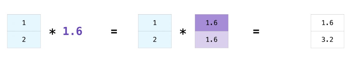
temps

[68, 72, 65, 64, 62, 61, 59, 64, 64, 63, 65, 62]

temp_array = np.array(temps)

# Increase all temperatures by 3 degrees.
temp_array + 3

array([71, 75, 68, 67, 65, 64, 62, 67, 67, 66, 68, 65])

# Halve all temperatures.
temp_array / 2

array([34. , 36. , 32.5, 32. , 31. , 30.5, 29.5, 32. , 32. , 31.5, 32.5,
       31. ])

# Convert all temperatures to Celsius.
(5 / 9) * (temp_array - 32)

array([20.  , 22.22, 18.33, 17.78, 16.67, 16.11, 15.  , 17.78, 17.78,
       17.22, 18.33, 16.67])

• Note: In none of the above cells did we actually modify temp_array! Each of those expressions created a new array. To actually change temp_array, we need to reassign it to a new array.

temp_array

array([68, 72, 65, 64, 62, 61, 59, 64, 64, 63, 65, 62])

temp_array = (5 / 9) * (temp_array - 32)

# Now in Celsius!
temp_array

array([20.  , 22.22, 18.33, 17.78, 16.67, 16.11, 15.  , 17.78, 17.78,
       17.22, 18.33, 16.67])

⚠️ The dangers of unnecessary for-loops

• Under the hood, numpy is implemented in C and Fortran, which are compiled languages that are much faster than Python. As a result, these vectorized operations are much quicker than if we used a vanilla Python for-loop.
  Also, the fact that arrays must be homogenous lend themselves to more efficient representations in memory.

• We can time code in a Jupyter Notebook. Let's try and square a long sequence of integers and see how long it takes with a Python loop:

%%timeit
squares = []
for i in range(1_000_000):
    squares.append(i * i)

46.5 ms ± 467 μs per loop (mean ± std. dev. of 7 runs, 10 loops each)

• In vanilla Python, this takes about 0.04 seconds per loop. In numpy:

%%timeit
squares = np.arange(1_000_000) ** 2

1.44 ms ± 50.3 μs per loop (mean ± std. dev. of 7 runs, 1,000 loops each)

• Only takes about 0.001 seconds per loop, more than 40x faster!

Element-wise arithmetic

• We can apply arithmetic operations to multiple arrays, provided they have the same length.
• The result is computed element-wise, which means that the arithmetic operation is applied to one pair of elements from each array at a time.

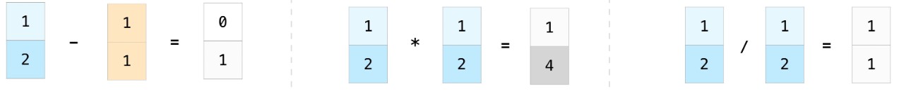
a = np.array([4, 5, -1])
b = np.array([2, 3, 2])

a + b

array([6, 8, 1])

a / b

array([ 2.  ,  1.67, -0.5 ])

a ** 2 + b ** 2

array([20, 34,  5])

Array methods

Arrays come equipped with several handy methods; some examples are below, but you can read about them all here.

arr = np.array([3, 8, 4, -3.2])

(2 ** arr).sum()

280.108818820412

(2 ** arr).mean()

70.027204705103

(2 ** arr).max()

256.0

(2 ** arr).argmax()

1

# An attribute, not a method.
arr.shape

(4,)

Next time

• We'll discuss how to work with 2D numpy arrays, and use it as an opportunity to review linear algebra.
  • Applications: Image filtering, Google PageRank.
• We'll then learn how to work with tabular data in pandas DataFrames.