from lec_utils import *

Lecture 15

Multiple Linear Regression

EECS 398: Practical Data Science, Winter 2025

practicaldsc.org • github.com/practicaldsc/wn25 • 📣 See latest announcements here on Ed

Agenda

• Regression and linear algebra.
• Multiple linear regression.
• Regression in sklearn.

Today's lecture is back to being in a notebook, but is still quite math heavy.

Question 🤔 (Answer at practicaldsc.org/q)

Remember that you can always ask questions anonymously at the link above!

Regression and linear algebra

---

The big picture

• Suppose we want to fit a simple linear regression model, $H(x_i) = w_0 + w_1 x_i$.

• Goal: Find the values of $w_0^*$ and $w_1^*$ that minimize mean squared error:

$$R_\text{sq}(w_0, w_1) = \frac{1}{n} \sum_{i = 1}^n (y_i - (w_0 + w_1 x_i))^2$$

• We've already done this using calculus. By formulating $R_\text{sq}$ in terms of matrices and vectors, we'll be able to extend our reasoning to models that use multiple input variables (the model above just uses one).

Terminology recap

• Define the design matrix $X \in \mathbb{R}^{n \times 2}$, observation vector $\vec y \in \mathbb{R}^n$, and parameter vector $\vec w \in \mathbb{R}^2$ as follows:

$$X = \begin{bmatrix} 1 & x_1 \\ 1 & x_2 \\ \vdots & \vdots \\ 1 & x_n \end{bmatrix} \qquad \vec y = \underbrace{\begin{bmatrix} y_1 \\ y_2 \\ \vdots \\ y_n \end{bmatrix}}_\text{vector of actual $y$ values} \qquad \vec{w} = \begin{bmatrix} w_0 \\ w_1 \end{bmatrix}$$

• Define the hypothesis vector, $\vec{h}$, as follows:

$$\vec h = \underbrace{\begin{bmatrix} H(x_1) \\ H(x_2) \\ \vdots \\ H(x_n) \end{bmatrix}}_\text{vector of predicted $y$ values} = \begin{bmatrix} w_0 + w_1 x_1 \\ w_0 + w_1 x_2 \\ \vdots \\ w_0 + w_1 x_n \end{bmatrix} = \underbrace{X \vec w}_\text{matrix-vector multiplication!}$$

Rewriting mean squared error

• The mean squared error of the predictions in $\vec h$ is:

$$\begin{align*} R_\text{sq}(w_0, w_1) &= \frac{1}{n} \sum_{i = 1}^n (y_i - (w_0 + w_1 x_i))^2 \end{align*}$$

• Equivalently, we have:

$$R_\text{sq}(\vec w) = \frac{1}{n} \lVert \vec y - \underbrace{X \vec w}_{\vec h} \rVert^2$$

• Which vector, $\vec w^*$, minimizes $R_\text{sq}(\vec w)$?
  

Equivalently, which vector $\vec w^*$ makes $\vec h = X \vec w^*$ as close to $\vec y$ as possible?

Geometric intuition

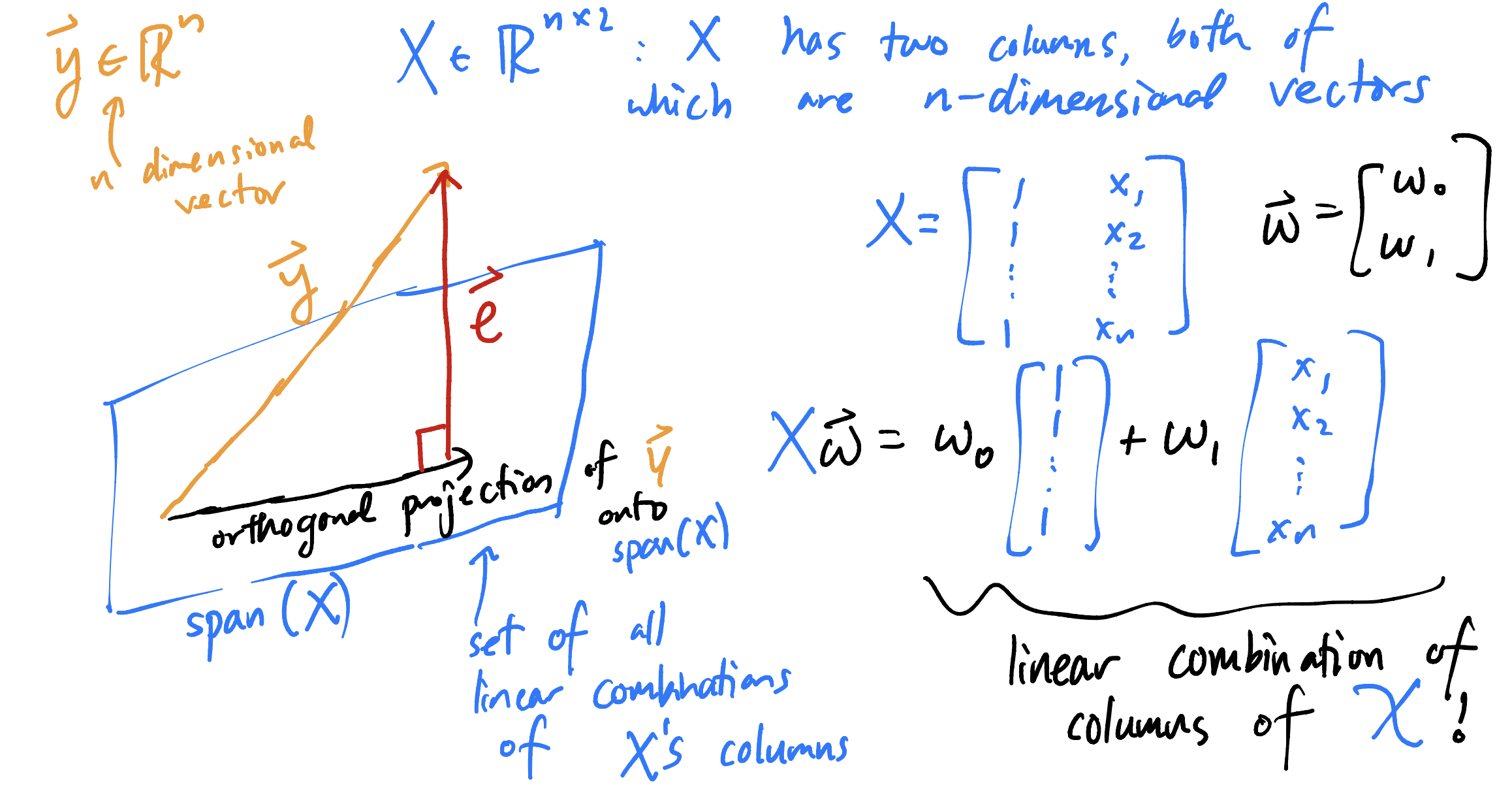
• Let $\vec e = \vec y - X \vec w$ be the error vector corresponding to the hypothesis vector $\vec h = X \vec w$.

• To make $X \vec w$ as close to $\vec y$ as possible, choose $\vec w^*$ such that:

$$\boxed{\text{the error vector}, \: \vec e = \vec y - X \vec w^*, \: \text{is orthogonal to the columns of} \: X!}$$

• In other words, we choose $\vec w^*$ such that $X \vec w^*$ is the orthogonal projection of $\vec y$ onto the span of the columns of $X$.

Minimizing mean squared error

• To minimize mean squared error, $R_\text{sq}(\vec w) = \frac{1}{n} \lVert \vec y - X \vec w \rVert^2$, we must choose the $\vec w^*$ such that the error vector, $\vec e = \vec y - X \vec w^*$, is orthogonal to the columns of $X$.

• Equivalently, we have:

  $$X^T \vec e = 0$$

  What are the dimensions of $X^T \vec e$?

• Expanding, we have:

$$\begin{align*} X^T (\vec y - X \vec w^*) &= 0 \\ X^T \vec y - X^TX \vec w^* &= 0 \\ X^T X \vec w^* &= X^T \vec y \end{align*}$$

• Key idea: The $\vec{w}^*$ that satisfies the last line above is the $\vec w^*$ that minimizes $R_\text{sq}(\vec{w})$!

The normal equations

• From the last slide, we have that the $\vec w^*$ that minimizes $R_\text{sq}(\vec w)$ is the $\vec w^*$ that satisfies the normal equations:

$$\boxed{X^TX \vec w^* = X^T \vec y}$$

• The normal equations are a system of two equations in two unknowns ($w_0$ and $w_1$).

• If $X^TX$ is invertible, there is a unique solution to the normal equations:

  $$\vec{w}^* = ({X^TX})^{-1} X^T \vec y$$

• If $X^TX$ is not invertible, then there are infinitely many solutions to the normal equations. We will explore this idea as the semester progresses.

The optimal parameter vector, $\vec{w}^*$

• To find the optimal model parameters for simple linear regression, $w_0^*$ and $w_1^*$, we previously minimized

$$R_\text{sq}(w_0, w_1) = \frac{1}{n} \sum_{i = 1}^n ({ y_i} - (w_0 + w_1 { x_i}))^2$$

• We found, using calculus, that:
  • $\boxed{w_1^* = \frac{\sum_{i = 1}^n (x_i - \bar{x})(y_i - \bar{y})}{\sum_{i = 1}^n (x_i - \bar{x})^2} = r \frac{\sigma_y}{\sigma_x}}$.
  • $\boxed{w_0^* = \bar{y} - w_1^* \bar{x}}$.

• Another way of finding optimal model parameters for simple linear regression is to find the $\vec{w}^*$ that minimizes $R_\text{sq}(\vec{w}) = \frac{1}{n} \lVert \vec y - X \vec w \rVert^2$.

• The minimizer, if $X^TX$ is invertible, is the vector $\boxed{\vec w^* = (X^TX)^{-1}X^T \vec y}$.
  If not, solve the normal equations from the previous slide.

• These $\boxed{\text{formulas}}$ are equivalent!

Multiple linear regression

---

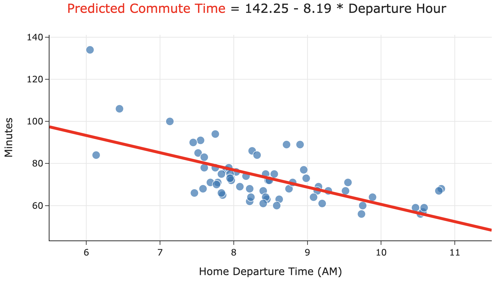
So far, we've fit simple linear regression models, which use only one feature ('departure_hour') for making predictions.

Incorporating multiple features

• In the context of the commute times dataset, the simple linear regression model we fit was of the form:

$$\begin{align*}\text{pred. commute} &= H(\text{departure hour}_i) \\ &= w_0 + w_1 \cdot \text{departure hour}_i \end{align*}$$

• Now, we'll try and fit a multiple linear regression model of the form:

$$\begin{align*}\text{pred. commute} &= H(\text{departure hour}_i, \text{day of month}_i) \\ &= w_0 + w_1 \cdot \text{departure hour}_i + w_2 \cdot \text{day of month}_i \end{align*}$$

• Linear regression with multiple features is called multiple linear regression.

• How do we find $w_0^*$, $w_1^*$, and $w_2^*$?

Geometric interpretation

• The hypothesis function:

  $$H(\text{departure hour}_i) = w_0 + w_1 \cdot \text{departure hour}_i$$

  looks like a line in 2D.

• Questions:

  • How many dimensions do we need to graph the hypothesis function:

  $$H(\text{departure hour}_i, \text{day of month}_i) = w_0 + w_1 \cdot \text{departure hour}_i + w_2 \cdot \text{day of month}_i$$

  • What is the shape of the hypothesis function?

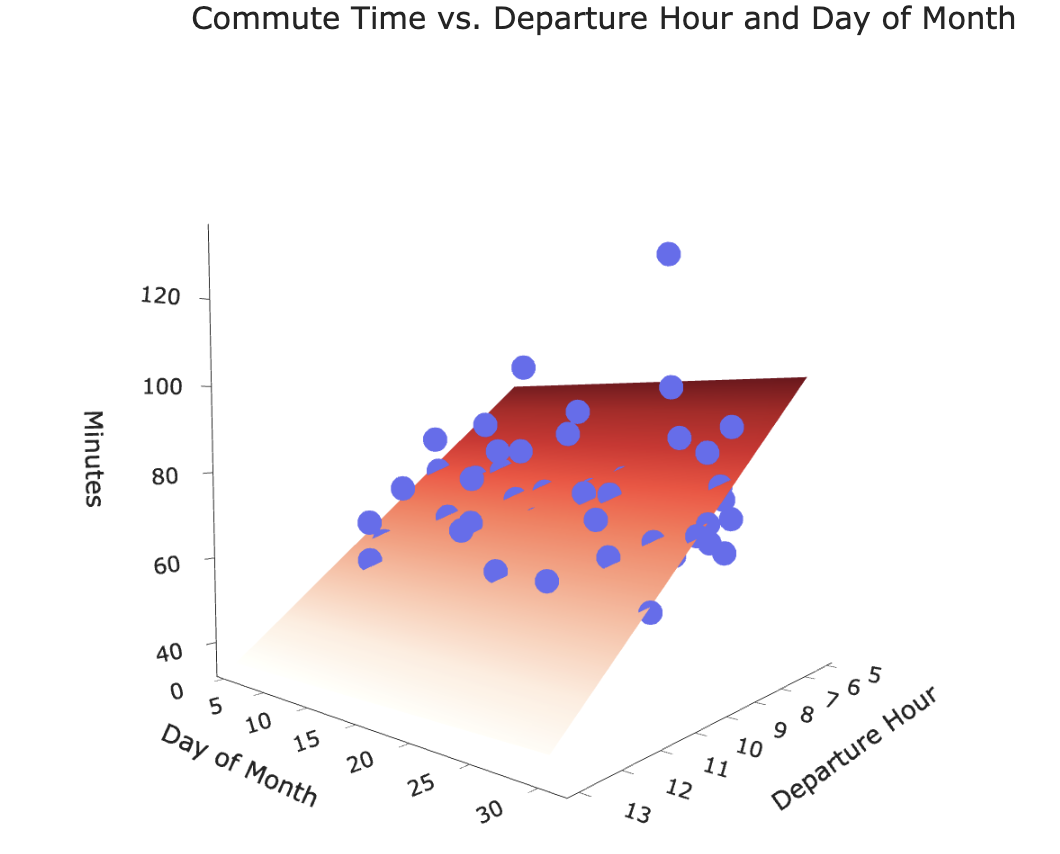
Our new hypothesis function is a plane in 3D!
Our goal is to find the plane of best fit that pierces through the cloud of points.

The hypothesis vector

• When our hypothesis function is of the form:

  $$H(\text{departure hour}) = w_0 + w_1 \cdot \text{departure hour} + w_2 \cdot \text{day of month}$$

  the hypothesis vector $\vec h \in \mathbb{R}^n$ can be written as:

$$\vec h = \begin{bmatrix} H(\text{departure hour}_1, \text{day}_1) \\ H(\text{departure hour}_2, \text{day}_2) \\ ... \\ H(\text{departure hour}_n, \text{day}_n) \\ \end{bmatrix} = \underbrace{\begin{bmatrix} 1 & \text{departure hour}_1 & \text{day}_1 \\ 1 & \text{departure hour}_2 & \text{day}_2 \\ ... & ... & ... \\ 1 & \text{departure hour}_n & \text{day}_n \end{bmatrix}}_{\text{3 columns!}} \begin{bmatrix} w_0 \\ w_1 \\ w_2 \end{bmatrix} $$

Finding the optimal parameters

• To find the optimal parameter vector, $\vec{w}^*$, we can use the design matrix $ X \in \mathbb{R}^{n \times 3}$ and observation vector $ \vec y \in \mathbb{R}^n$:

$$ X = \begin{bmatrix} 1 & \text{departure hour}_1 & \text{day}_1 \\ 1 & \text{departure hour}_2 & \text{day}_2 \\ ... & ... & ... \\ 1 & \text{departure hour}_n & \text{day}_n \end{bmatrix} \qquad \vec{y} = \begin{bmatrix} \text{commute time}_1 \\ \text{commute time}_2 \\ \vdots \\ \text{commute time}_n \end{bmatrix}$$

• Then, all we need to do is solve the normal equations once again:

  $$X^TX \vec{w}^* = X^T \vec y$$

  If $X^TX$ is invertible, we know the solution is:

$$\vec w^* = (X^TX)^{-1} X^T \vec y$$

• Let's generalize this notion beyond just two features.

Notation for multiple linear regression

• We will need to keep track of multiple features for every individual in our dataset.
  In practice, we could have hundreds, millions, or billions of features!

• As before, subscripts distinguish between individuals in our dataset. We have $n$ individuals, also called training examples.

• Superscripts distinguish between features. We have $d$ features.

  $$\text{departure hour}_i: \:\: x_i^{(1)}$$

  $$\text{day of month}_i: \:\: x_i^{(2)}$$

  Think of $x^{(1)}$, $x^{(2)}$, ... as new variable names, like new letters.

Feature vectors

• Suppose we have the following dataset.

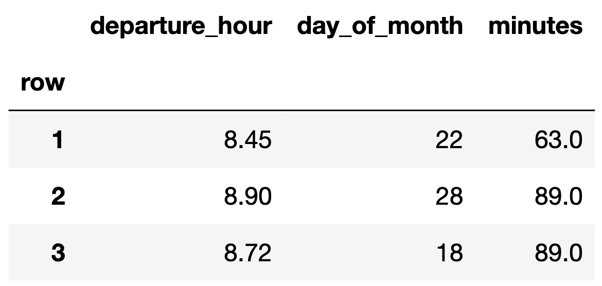
• We can represent each day with a feature vector, $\vec x_i = \begin{bmatrix} x_i^{(1)} \\ x_i^{(2)} \end{bmatrix}$:

$$ \vec x_1 = \begin{bmatrix} 8.45 \\ 22 \end{bmatrix} \qquad \vec x_2 = \begin{bmatrix} 8.90 \\ 28 \end{bmatrix} \qquad \vec x_2 = \begin{bmatrix} 8.72 \\ 18 \end{bmatrix}$$

Augmented feature vectors

• The augmented feature vector $\text{Aug}({\vec x_i})$ is the vector obtained by adding a 1 to the front of feature vector $\vec x_i$:

$$ { \vec x = \begin{bmatrix} {x^{(1)}} \\ {x^{(2)}} \\ \vdots \\ {x^{(d)}} \end{bmatrix} \qquad \text{Aug}({ \vec x}) = \begin{bmatrix} 1 \\ {x^{(1)}} \\ {x^{(2)}} \\ \vdots \\ { x^{(d)}} \end{bmatrix}} \qquad \vec w = \begin{bmatrix} w_0 \\ w_1 \\ w_2\\ \vdots \\ w_d \end{bmatrix} $$

• For example, if $\vec x_1 = \begin{bmatrix} 8.45 \\ 22 \end{bmatrix}$, then $\text{Aug}({\vec x_1}) = {\begin{bmatrix} 1 \\ 8.45 \\ 22 \end{bmatrix}}$.

• Then, our hypothesis function for individual $i$ is:

$$H({\vec x_i}) = w_0 + w_1 { x_i^{(1)}} + w_2 { x_i^{(2)}} + \ldots + w_d { x_i^{(d)}} = \vec w \cdot \text{Aug}({ \vec x_i})$$

The general problem

• We have $n$ data points, $\left({ \vec x_1}, {y_1}\right), \left({ \vec x_2}, {y_2}\right), \ldots, \left({ \vec x_n}, {y_n}\right)$,

where each $ \vec x_i$ is a feature vector of $d$ features: $${\vec{x_i}} = \begin{bmatrix} {x^{(1)}_i} \\ {x^{(2)}_i} \\ \vdots \\ {x^{(d)}_i} \end{bmatrix}$$

• We want to find a good linear hypothesis function:

$$H({\vec x_i}) = w_0 + w_1 { x_i^{(1)}} + w_2 { x_i^{(2)}} + \ldots + w_d { x_i^{(d)}} = \vec w \cdot \text{Aug}({ \vec x_i})$$

• Specifically, we want to find the optimal parameters, $w_0^*$, $w_1^*$, ..., $w_d^*$ that minimize mean squared error:

$$\begin{align*} R_\text{sq}(\vec w) &= \frac{1}{n} \sum_{i = 1}^n (y_i - H(\vec x_i))^2 \\ &= \frac{1}{n} \sum_{i = 1}^n \left( y_i - (w_0 + w_1 { x_i^{(1)}} + w_2 { x_i^{(2)}} + \ldots + w_d { x_i^{(d)}})\right)^2 \\ &= \frac{1}{n} \sum_{i = 1}^n \left(y_i - \text{Aug}(\vec x_i) \cdot \vec{w} \right)^2 \\ &= \frac{1}{n} \lVert \vec y - X \vec w \rVert^2 \end{align*}$$

The general solution

• Define the design matrix $ X \in \mathbb{R}^{n \times (d + 1)}$ and observation vector $\vec y \in \mathbb{R}^n$:

$${ X= \begin{bmatrix} {1} & { x^{(1)}_1} & { x^{(2)}_1} & \dots & { x^{(d)}_1} \\\\ { 1} & { x^{(1)}_2} & { x^{(2)}_2} & \dots & { x^{(d)}_2} \\\\ \vdots & \vdots & \vdots & & \vdots \\\\ { 1} & { x^{(1)}_n} & { x^{(2)}_n} & \dots & { x^{(d)}_n} \end{bmatrix} = \begin{bmatrix} \text{Aug}({\vec{x_1}})^T \\\\ \text{Aug}({\vec{x_2}})^T \\\\ \vdots \\\\ \text{Aug}({\vec{x_n}})^T \end{bmatrix}} \qquad { \vec y = \begin{bmatrix} { y_1} \\ { y_2} \\ \vdots \\ { y_n} \end{bmatrix}}$$

• Then, solve the normal equations to find the optimal parameter vector, $\vec{w}^*$:

$$X^TX \vec w^* = X^T \vec y$$

• The $\vec w^*$ that satisfies the equations above minimizes mean squared error, $R_\text{sq}(\vec w)$.

Note on parameters

• With $d$ features, $\vec w$ has $d+1$ entries.

• Again, $\vec w^*$ represents our optimal parameter vector, that minimizes mean squared error.

• $w_0^*$ is the bias, also known as the intercept.

• $w_1^*, w_2^*, ... , w_d^*$ each give the weight, or coefficient, or slope, of a feature.

$$H({\vec x_i}) = w_0 + w_1 { x_i^{(1)}} + w_2 { x_i^{(2)}} + \ldots + w_d { x_i^{(d)}} = \vec w \cdot \text{Aug}({ \vec x_i})$$

Question 🤔 (Answer at practicaldsc.org/q)

Remember that you can always ask questions anonymously at the link above!

Regression in sklearn

---

Loading the data

• Run the cell below to load in our commute times dataset.

df = pd.read_csv('data/commute-times.csv')
df['day_of_month'] = pd.to_datetime(df['date']).dt.day
df.head()

	date	day	home_departure_time	home_departure_mileage	...	minutes_to_home	work_departure_time_hr	mileage_to_home	day_of_month
0	5/15/2023	Mon	2023-05-15 10:49:00	15873.0	...	72.0	17.17	53.0	15
1	5/16/2023	Tue	2023-05-16 07:45:00	15979.0	...	NaN	NaN	NaN	16
2	5/22/2023	Mon	2023-05-22 08:27:00	50407.0	...	82.0	15.90	54.0	22
3	5/23/2023	Tue	2023-05-23 07:08:00	50535.0	...	NaN	NaN	NaN	23
4	5/30/2023	Tue	2023-05-30 09:09:00	50664.0	...	76.0	17.12	54.0	30

5 rows × 19 columns

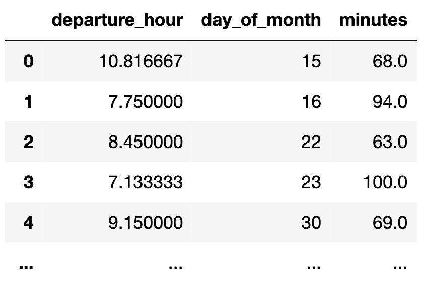
• For now, the only relevant columns for us are 'departure_hour', 'day_of_month', and 'minutes'.

df[['departure_hour', 'day_of_month', 'minutes']]

	departure_hour	day_of_month	minutes
0	10.82	15	68.0
1	7.75	16	94.0
2	8.45	22	63.0
...	...	...	...
62	7.58	4	68.0
63	7.45	5	90.0
64	7.60	7	83.0

65 rows × 3 columns

sklearn

• sklearn (scikit-learn) implements many common steps in the feature and model creation pipeline.
  It is widely used throughout industry and academia.

• It interfaces with numpy arrays, and to an extent, pandas DataFrames.

• Huge benefit: the documentation online is excellent.

The LinearRegression class

• sklearn comes with several subpackages, including linear_model and tree, each of which contains several classes of models.

• We'll start with the LinearRegression class from linear_model.

from sklearn.linear_model import LinearRegression

• Important: From the documentation, we have:

LinearRegression fits a linear model with coefficients w = (w1, …, wp) to minimize the residual sum of squares between the observed targets in the dataset, and the targets predicted by the linear approximation.

In other words, **`LinearRegression` minimizes mean squared error by default**! (Per the documentation, it also includes an intercept term by default.)

LinearRegression?

Fitting a multiple linear regression model

• Let's aim to use sklearn to find the optimal parameters for the following model:

$$\begin{align*}\text{pred. commute} &= H(\text{departure hour}_i, \text{day of month}_i) \\ &= w_0 + w_1 \cdot \text{departure hour}_i + w_2 \cdot \text{day of month}_i \end{align*}$$

• First, we must instantiate a LinearRegression object and fit it. By calling fit, we are saying "minimize mean squared error on this dataset and find $w^*$."

model_multiple = LinearRegression()
# Note that there are two arguments to fit – X and y!
# (It is not necessary to write X= and y=)
model_multiple.fit(X=df[['departure_hour', 'day_of_month']], y=df['minutes'])

LinearRegression()

In a Jupyter environment, please rerun this cell to show the HTML representation or trust the notebook.
On GitHub, the HTML representation is unable to render, please try loading this page with nbviewer.org.

• After fitting, we can access $w^*$ – that is, the best intercept and coefficients.

model_multiple.intercept_, model_multiple.coef_ 

(141.86402699471932, array([-8.22,  0.06]))

• These coefficients tell us that the "best way" (according to squared loss) to make commute time predictions using a linear model is using:

$$\text{pred. commute}_i = 141.86 - 8.22 \cdot \text{departure hour}_i + 0.06 \cdot \text{day of month}_i$$

• This is the plane of best fit given historical data; it is not a causal statement.

Let's visualize this model.

XX, YY = np.mgrid[5:14:1, 0:31:1]
Z = model_multiple.intercept_ + model_multiple.coef_[0] * XX + model_multiple.coef_[1] * YY
plane = go.Surface(x=XX, y=YY, z=Z, colorscale='Reds')
fig = go.Figure(data=[plane])
fig.add_trace(go.Scatter3d(x=df['departure_hour'], 
                           y=df['day_of_month'], 
                           z=df['minutes'], mode='markers', marker = {'color': '#656DF1'}))
fig.update_layout(scene=dict(xaxis_title='Departure Hour',
                             yaxis_title='Day of Month',
                             zaxis_title='Minutes'),
                  title='Commute Time vs. Departure Hour and Day of Month',
                  width=1000, height=500)

Making predictions

• Fit LinearRegression objects also have a predict method, which can be used to predict commute times given a 'departure_hour' and 'day_of_month'.

# What if I leave at 9:15AM on the 26th of the month?
model_multiple.predict([[9.25, 26]]) 

array([67.26])

model_multiple.predict(pd.DataFrame({'departure_hour': [9.25], 'day_of_month': [26]}))

array([67.26])

Comparing models

• Since we're going to start to fit lots of different models to the commute times dataset, it'll be useful to compare their mean squared errors.

• sklearn has a built-in mean_squared_error function.
  Remember, the units of MSE are the units of $y$, squared. So the value below is 96.78 $\text{minutes}^2$.

from sklearn.metrics import mean_squared_error

mean_squared_error(df['minutes'], model_multiple.predict(df[['departure_hour', 'day_of_month']])) 

96.78730488437492

• Let's construct a dictionary to keep track of the MSEs we've seen so far.

mse_dict = {}
mse_dict['departure_hour + day_of_month'] = mean_squared_error(df['minutes'], model_multiple.predict(df[['departure_hour', 'day_of_month']]))

• To compare, let's also fit and measure a simple linear model and constant model.

# Simple linear model.
model_simple = LinearRegression()
model_simple.fit(X=df[['departure_hour']], y=df['minutes'])
mse_dict['departure_hour'] = mean_squared_error(df['minutes'], model_simple.predict(df[['departure_hour']]))

# Constant model.
model_constant = df['minutes'].mean()
mse_dict['constant'] = mean_squared_error(df['minutes'], np.ones(df.shape[0]) * model_constant)

• As we can see, adding 'day_of_month' as a feature barely reduced our model's MSE.
  Next week, when we learn about generalization, we'll see why sometimes adding more features is a bad thing!

mse_dict

{'departure_hour + day_of_month': 96.78730488437492,
 'departure_hour': 97.04687150819183,
 'constant': 167.535147928994}

LinearRegression class summary

Property	Example	Description
Initialize model parameters	lr = LinearRegression()	Create (empty) linear regression model
Fit the model to the data	lr.fit(X, y)	Determines regression coefficients
Use model for prediction	lr.predict(X_new)	Uses regression line to make predictions
Access model attributes	lr.coef_, lr.intercept_	Accesses the regression coefficients and intercept

What's next?

• So far, in our journey to predict 'minutes', we've only used two numerical features in our dataset, 'departure_hour' and 'day_of_month'.

df[['departure_hour', 'day_of_month', 'minutes']]

	departure_hour	day_of_month	minutes
0	10.82	15	68.0
1	7.75	16	94.0
2	8.45	22	63.0
...	...	...	...
62	7.58	4	68.0
63	7.45	5	90.0
64	7.60	7	83.0

65 rows × 3 columns

• There's a lot of information in df that we didn't use –'day', for example. We can't use these 'day' in it's current form as it's non-numeric.

• How do we use categorical features in a regression model?