from lec_utils import *
def show_merging_animation():
    src = "https://docs.google.com/presentation/d/1HPJ7fiBLNEURsWYiY0qpqPR3qup68Mr0_B34GU99Y8Q/embed?start=false&loop=false&delayms=60000&rm=minimal"
    width = 865
    height = 509
    display(IFrame(src, width, height))
Lecture 6
Pivoting, Merging, and Transforming
EECS 398: Practical Data Science, Winter 2025
practicaldsc.org • github.com/practicaldsc/wn25 • 📣 See latest announcements here on Ed
3blue1bron 🏀
- 3blue1bron allows you to upload a PDF and it'll automatically generate a video of LeBron James summarizing the notes.
- Listen up! 🐐
IFrame(
    src='https://www.3blue1bron.com/share/7c278b09-f703-454c-9e23-31564f38b040',
    width=800,
    height=700
)
Agenda 📆
- Recap:
groupby. - Pivot tables using
pivot_table. - Merging 🚗.
- Transforming 🤖.
Recap: groupby
Loading the data 🐧

penguins = pd.read_csv('data/penguins.csv')
penguins
| species | island | bill_length_mm | bill_depth_mm | flipper_length_mm | body_mass_g | sex | |
|---|---|---|---|---|---|---|---|
| 0 | Adelie | Dream | 41.3 | 20.3 | 194.0 | 3550.0 | Male |
| 1 | Adelie | Torgersen | 38.5 | 17.9 | 190.0 | 3325.0 | Female |
| 2 | Adelie | Dream | 34.0 | 17.1 | 185.0 | 3400.0 | Female |
| ... | ... | ... | ... | ... | ... | ... | ... |
| 330 | Chinstrap | Dream | 46.6 | 17.8 | 193.0 | 3800.0 | Female |
| 331 | Adelie | Dream | 39.7 | 17.9 | 193.0 | 4250.0 | Male |
| 332 | Gentoo | Biscoe | 45.1 | 14.5 | 207.0 | 5050.0 | Female |
333 rows × 7 columns
The groupby method
- The
groupbymethod helps us answer questions that involve performing some computation separately for each group.
- Most commonly, we'll use
groupby, select column(s) to operate on, and use a built-in aggregation method.
# The median 'bill_length_mm' of each 'species'.
penguins.groupby('species')['bill_length_mm'].median()
species
Adelie       38.85
Chinstrap    49.55
Gentoo       47.40
Name: bill_length_mm, dtype: float64
- There are four other special "grouping methods" we learned about last class that allow for advanced behavior, namely
agg,filter,transform, andapply.
See "⭐️ The grouping method cheat sheet" from last lecture for examples.
# The most common 'island' per 'species'.
penguins.groupby('species')['island'].agg(lambda s: s.value_counts().idxmax())
species
Adelie        Dream
Chinstrap     Dream
Gentoo       Biscoe
Name: island, dtype: object
# Keeps the 'species' with at least 100 penguins.
penguins.groupby('species').filter(lambda df: df.shape[0] >= 100)
| species | island | bill_length_mm | bill_depth_mm | flipper_length_mm | body_mass_g | sex | |
|---|---|---|---|---|---|---|---|
| 0 | Adelie | Dream | 41.3 | 20.3 | 194.0 | 3550.0 | Male |
| 1 | Adelie | Torgersen | 38.5 | 17.9 | 190.0 | 3325.0 | Female |
| 2 | Adelie | Dream | 34.0 | 17.1 | 185.0 | 3400.0 | Female |
| ... | ... | ... | ... | ... | ... | ... | ... |
| 326 | Adelie | Dream | 41.1 | 18.1 | 205.0 | 4300.0 | Male |
| 331 | Adelie | Dream | 39.7 | 17.9 | 193.0 | 4250.0 | Male |
| 332 | Gentoo | Biscoe | 45.1 | 14.5 | 207.0 | 5050.0 | Female |
265 rows × 7 columns
Grouping with multiple columns
- When we group with multiple columns, one group is created for every unique combination of elements in the specified columns.
In the output below, why are there only 5 rows, rather than $3 \times 3 = 9$ rows, when there are 3 unique'species'and 3 unique'island's?
# Read this as:
species_and_island = (
    penguins.groupby(['species', 'island'])         # for every combination of 'species' and 'island' in the DataFrame,
    [['bill_length_mm', 'bill_depth_mm']].mean()    # calculate the mean 'bill_length_mm' and the mean 'bill_depth_mm'.
)
species_and_island
| bill_length_mm | bill_depth_mm | ||
|---|---|---|---|
| species | island | ||
| Adelie | Biscoe | 38.98 | 18.37 |
| Dream | 38.52 | 18.24 | |
| Torgersen | 39.04 | 18.45 | |
| Chinstrap | Dream | 48.83 | 18.42 |
| Gentoo | Biscoe | 47.57 | 15.00 |
- Advice: When grouping on multiple columns, the result usually has a
MultiIndex; usereset_indexor setas_index=Falseingroupbyto avoid this.
# Now, this looks like a regular DataFrame!
species_and_island.reset_index()
| species | island | bill_length_mm | bill_depth_mm | |
|---|---|---|---|---|
| 0 | Adelie | Biscoe | 38.98 | 18.37 |
| 1 | Adelie | Dream | 38.52 | 18.24 |
| 2 | Adelie | Torgersen | 39.04 | 18.45 |
| 3 | Chinstrap | Dream | 48.83 | 18.42 |
| 4 | Gentoo | Biscoe | 47.57 | 15.00 |
Pivot tables using pivot_table
Pivot tables: An extension of grouping
- Pivot tables are a compact way to display tables for humans to read.
| sex | Female | Male |
|---|---|---|
| species | ||
| Adelie | 3368.84 | 4043.49 |
| Chinstrap | 3527.21 | 3938.97 |
| Gentoo | 4679.74 | 5484.84 |
- Notice that each value in the table is the average of
'body_mass_g'of penguins, for every combination of'species'and'sex'.
- You can think of pivot tables as grouping using two columns, then "pivoting" one of the group labels into columns.
pivot_table
- The
pivot_tableDataFrame method aggregates a DataFrame using two columns. To use it:
df.pivot_table(index=index_col,
                       columns=columns_col,
                       values=values_col,
                       aggfunc=func)
- The resulting DataFrame will have:
- One row for every unique value in
index_col. - One column for every unique value in
columns_col. - Values determined by applying
funcon values invalues_col.
- One row for every unique value in
- Example: Find the average
'body_mass_g'for every combination of'species'and'sex'.
penguins.pivot_table(
    index='species',
    columns='sex',
    values='body_mass_g',
    aggfunc='mean'
)
| sex | Female | Male |
|---|---|---|
| species | ||
| Adelie | 3368.84 | 4043.49 |
| Chinstrap | 3527.21 | 3938.97 |
| Gentoo | 4679.74 | 5484.84 |
# Same information as above, but harder to read!
(
    penguins
    .groupby(['species', 'sex'])
    [['body_mass_g']]
    .mean()
)
| body_mass_g | ||
|---|---|---|
| species | sex | |
| Adelie | Female | 3368.84 |
| Male | 4043.49 | |
| Chinstrap | Female | 3527.21 |
| Male | 3938.97 | |
| Gentoo | Female | 4679.74 |
| Male | 5484.84 |
Example: Finding the number of penguins per 'island' and 'species'
penguins
| species | island | bill_length_mm | bill_depth_mm | flipper_length_mm | body_mass_g | sex | |
|---|---|---|---|---|---|---|---|
| 0 | Adelie | Dream | 41.3 | 20.3 | 194.0 | 3550.0 | Male |
| 1 | Adelie | Torgersen | 38.5 | 17.9 | 190.0 | 3325.0 | Female |
| 2 | Adelie | Dream | 34.0 | 17.1 | 185.0 | 3400.0 | Female |
| ... | ... | ... | ... | ... | ... | ... | ... |
| 330 | Chinstrap | Dream | 46.6 | 17.8 | 193.0 | 3800.0 | Female |
| 331 | Adelie | Dream | 39.7 | 17.9 | 193.0 | 4250.0 | Male |
| 332 | Gentoo | Biscoe | 45.1 | 14.5 | 207.0 | 5050.0 | Female |
333 rows × 7 columns
- Suppose we want to find the number of penguins in
penguinsper'island'and'species'. We can do so withoutpivot_table:
penguins.value_counts(['island', 'species'])
island     species
Biscoe     Gentoo       119
Dream      Chinstrap     68
           Adelie        55
Torgersen  Adelie        47
Biscoe     Adelie        44
Name: count, dtype: int64
penguins.groupby(['island', 'species']).size()
island     species
Biscoe     Adelie        44
           Gentoo       119
Dream      Adelie        55
           Chinstrap     68
Torgersen  Adelie        47
dtype: int64
- But the data is arguably easier to interpret when we do use
pivot_table:
penguins.pivot_table(
    index='species',
    columns='island',
    values='bill_length_mm', # Choice of column here doesn't actually matter! Why?
    aggfunc='count',
)
| island | Biscoe | Dream | Torgersen |
|---|---|---|---|
| species | |||
| Adelie | 44.0 | 55.0 | 47.0 |
| Chinstrap | NaN | 68.0 | NaN |
| Gentoo | 119.0 | NaN | NaN |
- Note that there is a
NaNat the intersection of'Biscoe'and'Chinstrap', because there were no Chinstrap penguins on Biscoe Island.NaNstands for "not a number." It isnumpyandpandas' version of a null value (the regular Python null value isNone). We'll learn more about how to deal with these soon.
- We can either use the
fillnamethod afterwards or thefill_valueargument to fill inNaNs.
penguins.pivot_table(
    index='species',
    columns='island',
    values='bill_length_mm',
    aggfunc='count',
    fill_value=0,
)
| island | Biscoe | Dream | Torgersen |
|---|---|---|---|
| species | |||
| Adelie | 44 | 55 | 47 |
| Chinstrap | 0 | 68 | 0 |
| Gentoo | 119 | 0 | 0 |
Granularity
- Each row of the original
penguinsDataFrame represented a single penguin, and each column represented features of the penguins.
penguins
| species | island | bill_length_mm | bill_depth_mm | flipper_length_mm | body_mass_g | sex | |
|---|---|---|---|---|---|---|---|
| 0 | Adelie | Dream | 41.3 | 20.3 | 194.0 | 3550.0 | Male |
| 1 | Adelie | Torgersen | 38.5 | 17.9 | 190.0 | 3325.0 | Female |
| 2 | Adelie | Dream | 34.0 | 17.1 | 185.0 | 3400.0 | Female |
| ... | ... | ... | ... | ... | ... | ... | ... |
| 330 | Chinstrap | Dream | 46.6 | 17.8 | 193.0 | 3800.0 | Female |
| 331 | Adelie | Dream | 39.7 | 17.9 | 193.0 | 4250.0 | Male |
| 332 | Gentoo | Biscoe | 45.1 | 14.5 | 207.0 | 5050.0 | Female |
333 rows × 7 columns
- What is the granularity of the DataFrame below?
That is, what does each row represent?
penguins.pivot_table(
    index='species',
    columns='island',
    values='bill_length_mm',
    aggfunc='count',
    fill_value=0,
)
| island | Biscoe | Dream | Torgersen |
|---|---|---|---|
| species | |||
| Adelie | 44 | 55 | 47 |
| Chinstrap | 0 | 68 | 0 |
| Gentoo | 119 | 0 | 0 |
Reshaping
pivot_tablereshapes DataFrames from "long" to "wide".
- Other DataFrame reshaping methods:
melt: Un-pivots a DataFrame. Very useful in data cleaning. See the reference slide!pivot: Likepivot_table, but doesn't do aggregation.stack: Pivots multi-level columns to multi-indices.unstack: Pivots multi-indices to columns.
- Google, the documentation, and ChatGPT are your friends!
- The
meltmethod is common enough that we'll give it a special mention.
- We'll often encounter pivot tables (esp. from government data), which we call wide data.
- The methods we've introduced work better with long-form data, or tidy data.
- To go from wide to long,
melt.

wide_example = pd.DataFrame({
    'Year': [2001, 2002],
    'Jan': [10, 130],
    'Feb': [20, 200],
    'Mar': [30, 340]
}).set_index('Year')
wide_example
| Jan | Feb | Mar | |
|---|---|---|---|
| Year | |||
| 2001 | 10 | 20 | 30 |
| 2002 | 130 | 200 | 340 |
wide_example.melt(ignore_index=False)
| variable | value | |
|---|---|---|
| Year | ||
| 2001 | Jan | 10 |
| 2002 | Jan | 130 |
| 2001 | Feb | 20 |
| 2002 | Feb | 200 |
| 2001 | Mar | 30 |
| 2002 | Mar | 340 |
Merging 🚗
phones = pd.DataFrame().assign(
    Model=['iPhone 16', 'iPhone 16 Pro Max', 'Samsung Galaxy S24 Ultra', 'Pixel 9 Pro'],
    Price=[799, 1199, 1299, 999],
    Screen=[6.1, 6.9, 6.8, 6.3]
)
inventory = pd.DataFrame().assign(
    Handset=['iPhone 16 Pro Max', 'iPhone 16', 'Pixel 9 Pro', 'Pixel 9 Pro', 'iPhone 16', 'iPhone 15'],
    Units=[50, 40, 10, 15, 100, 5],
    Store=['Briarwood', 'Somerset', 'Arbor Hills', '12 Oaks', 'Briarwood', 'Oakland Mall']
)
Example: Phone sales 📱
# The DataFrame on the left contains information about phones on the market.
# The DataFrame on the right contains information about the stock I have in my stores.
dfs_side_by_side(phones, inventory)
| Model | Price | Screen | |
|---|---|---|---|
| 0 | iPhone 16 | 799 | 6.1 |
| 1 | iPhone 16 Pro Max | 1199 | 6.9 |
| 2 | Samsung Galaxy S24 Ultra | 1299 | 6.8 |
| 3 | Pixel 9 Pro | 999 | 6.3 |
| Handset | Units | Store | |
|---|---|---|---|
| 0 | iPhone 16 Pro Max | 50 | Briarwood |
| 1 | iPhone 16 | 40 | Somerset |
| 2 | Pixel 9 Pro | 10 | Arbor Hills |
| 3 | Pixel 9 Pro | 15 | 12 Oaks |
| 4 | iPhone 16 | 100 | Briarwood |
| 5 | iPhone 15 | 5 | Oakland Mall |
- Question: If I sell all of the phones in my inventory, how much will I make in revenue?
- The information I need to answer the question is spread across multiple DataFrames.
- The solution is to merge the two DataFrames together horizontally.
The SQL term for merge is join.
- A merge is appropriate when we have two sources of information about the same individuals that is linked by a common column(s).
The common column(s) are called the join key.
If I sell all of the phones in my inventory, how much will I make in revenue?
combined = phones.merge(inventory, left_on='Model', right_on='Handset')
combined
| Model | Price | Screen | Handset | Units | Store | |
|---|---|---|---|---|---|---|
| 0 | iPhone 16 | 799 | 6.1 | iPhone 16 | 40 | Somerset |
| 1 | iPhone 16 | 799 | 6.1 | iPhone 16 | 100 | Briarwood |
| 2 | iPhone 16 Pro Max | 1199 | 6.9 | iPhone 16 Pro Max | 50 | Briarwood |
| 3 | Pixel 9 Pro | 999 | 6.3 | Pixel 9 Pro | 10 | Arbor Hills |
| 4 | Pixel 9 Pro | 999 | 6.3 | Pixel 9 Pro | 15 | 12 Oaks |
(combined['Price'] * combined['Units']).sum()
196785
What just happened!? 🤯
# Click through the presentation that appears.
show_merging_animation()
The merge method
- The
mergeDataFrame method joins two DataFrames by columns or indexes.
As mentioned before, "merge" is just thepandasword for "join."
- When using the
mergemethod, the DataFrame beforemergeis the "left" DataFrame, and the DataFrame passed intomergeis the "right" DataFrame.
Inphones.merge(inventory),phonesis considered the "left" DataFrame andinventoryis the "right" DataFrame.
The columns from the left DataFrame appear to the left of the columns from right DataFrame.
- By default:
- If join keys are not specified, all shared columns between the two DataFrames are used.
- The "type" of join performed is an inner join, which is just one of many types of joins.
Inner joins
- The default type of join that
mergeperforms is an inner join, which keeps the intersection of the join keys.

# The DataFrame on the far right is the merged DataFrame.
dfs_side_by_side(phones, inventory, phones.merge(inventory, left_on='Model', right_on='Handset'))
| Model | Price | Screen | |
|---|---|---|---|
| 0 | iPhone 16 | 799 | 6.1 |
| 1 | iPhone 16 Pro Max | 1199 | 6.9 |
| 2 | Samsung Galaxy S24 Ultra | 1299 | 6.8 |
| 3 | Pixel 9 Pro | 999 | 6.3 |
| Handset | Units | Store | |
|---|---|---|---|
| 0 | iPhone 16 Pro Max | 50 | Briarwood |
| 1 | iPhone 16 | 40 | Somerset |
| 2 | Pixel 9 Pro | 10 | Arbor Hills |
| 3 | Pixel 9 Pro | 15 | 12 Oaks |
| 4 | iPhone 16 | 100 | Briarwood |
| 5 | iPhone 15 | 5 | Oakland Mall |
| Model | Price | Screen | Handset | Units | Store | |
|---|---|---|---|---|---|---|
| 0 | iPhone 16 | 799 | 6.1 | iPhone 16 | 40 | Somerset |
| 1 | iPhone 16 | 799 | 6.1 | iPhone 16 | 100 | Briarwood |
| 2 | iPhone 16 Pro Max | 1199 | 6.9 | iPhone 16 Pro Max | 50 | Briarwood |
| 3 | Pixel 9 Pro | 999 | 6.3 | Pixel 9 Pro | 10 | Arbor Hills |
| 4 | Pixel 9 Pro | 999 | 6.3 | Pixel 9 Pro | 15 | 12 Oaks |
- Note that
'Samsung Galaxy S24 Ultra'and'iPhone 15'do not appear in the merged DataFrame.
- That's because there is no
'Samsung Galaxy S24 Ultra'in the right DataFrame (inventory), and no'iPhone 15'in the left DataFrame (phones).
Other join types
- We can change the type of join performed by changing the
howargument inmerge.
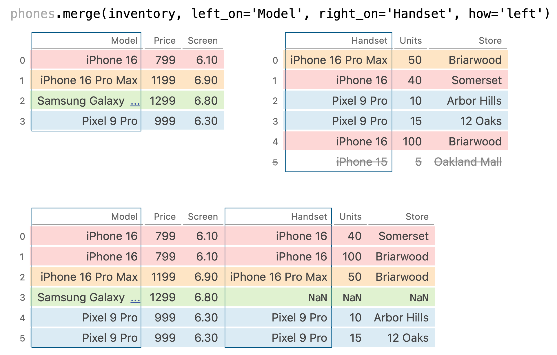
phones.merge(inventory, left_on='Model', right_on='Handset', how='left')
| Model | Price | Screen | Handset | Units | Store | |
|---|---|---|---|---|---|---|
| 0 | iPhone 16 | 799 | 6.1 | iPhone 16 | 40.0 | Somerset |
| 1 | iPhone 16 | 799 | 6.1 | iPhone 16 | 100.0 | Briarwood |
| 2 | iPhone 16 Pro Max | 1199 | 6.9 | iPhone 16 Pro Max | 50.0 | Briarwood |
| 3 | Samsung Galaxy S24 Ultra | 1299 | 6.8 | NaN | NaN | NaN |
| 4 | Pixel 9 Pro | 999 | 6.3 | Pixel 9 Pro | 10.0 | Arbor Hills |
| 5 | Pixel 9 Pro | 999 | 6.3 | Pixel 9 Pro | 15.0 | 12 Oaks |
phones.merge(inventory, left_on='Model', right_on='Handset', how='right')
| Model | Price | Screen | Handset | Units | Store | |
|---|---|---|---|---|---|---|
| 0 | iPhone 16 Pro Max | 1199.0 | 6.9 | iPhone 16 Pro Max | 50 | Briarwood |
| 1 | iPhone 16 | 799.0 | 6.1 | iPhone 16 | 40 | Somerset |
| 2 | Pixel 9 Pro | 999.0 | 6.3 | Pixel 9 Pro | 10 | Arbor Hills |
| 3 | Pixel 9 Pro | 999.0 | 6.3 | Pixel 9 Pro | 15 | 12 Oaks |
| 4 | iPhone 16 | 799.0 | 6.1 | iPhone 16 | 100 | Briarwood |
| 5 | NaN | NaN | NaN | iPhone 15 | 5 | Oakland Mall |
phones.merge(inventory, left_on='Model', right_on='Handset', how='outer')
| Model | Price | Screen | Handset | Units | Store | |
|---|---|---|---|---|---|---|
| 0 | iPhone 16 | 799.0 | 6.1 | iPhone 16 | 40.0 | Somerset |
| 1 | iPhone 16 | 799.0 | 6.1 | iPhone 16 | 100.0 | Briarwood |
| 2 | iPhone 16 Pro Max | 1199.0 | 6.9 | iPhone 16 Pro Max | 50.0 | Briarwood |
| 3 | Samsung Galaxy S24 Ultra | 1299.0 | 6.8 | NaN | NaN | NaN |
| 4 | Pixel 9 Pro | 999.0 | 6.3 | Pixel 9 Pro | 10.0 | Arbor Hills |
| 5 | Pixel 9 Pro | 999.0 | 6.3 | Pixel 9 Pro | 15.0 | 12 Oaks |
| 6 | NaN | NaN | NaN | iPhone 15 | 5.0 | Oakland Mall |
- The website pandastutor.com can help visualize DataFrame operations like these.
Here's a direct link to this specific example.
Different join types handle mismatches differently
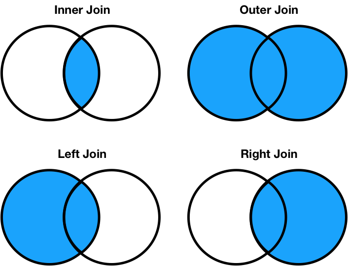
- Inner join: Keep only the matching keys (intersection).
- Outer join: Keep all keys in both DataFrames (union).
- Left join: Keep all keys in the left DataFrame, whether or not they are in the right DataFrame.
- Right join: Keep all keys in the right DataFrame, whether or not they are in the left DataFrame.
Note thata.merge(b, how='left')contains the same information asb.merge(a, how='right'), just in a different order.
Tip: Set differences
- A set in Python is a data structure containing unique, unordered elements.
phones['Model']
0                   iPhone 16
1           iPhone 16 Pro Max
2    Samsung Galaxy S24 Ultra
3                 Pixel 9 Pro
Name: Model, dtype: object
left = set(phones['Model'])
left
{'Pixel 9 Pro', 'Samsung Galaxy S24 Ultra', 'iPhone 16', 'iPhone 16 Pro Max'}
inventory['Handset']
0    iPhone 16 Pro Max
1            iPhone 16
2          Pixel 9 Pro
3          Pixel 9 Pro
4            iPhone 16
5            iPhone 15
Name: Handset, dtype: object
right = set(inventory['Handset'])
right
{'Pixel 9 Pro', 'iPhone 15', 'iPhone 16', 'iPhone 16 Pro Max'}
- To quickly check which join key values are in the left DataFrame but not the right, or vice versa, create sets out of the join keys and use the
differencemethod.
left.difference(right)
{'Samsung Galaxy S24 Ultra'}
right.difference(left)
{'iPhone 15'}
mergeis flexible – you can merge using a combination of columns, or the index of the DataFrame.
- If the two DataFrames have the same column names,
pandaswill add_xand_yto the duplicated column names to avoid having columns with the same name (change these thesuffixesargument).
- There is, in fact, a
joinmethod, but it's actually a wrapper aroundmergewith fewer options.
- As always, the documentation is your friend!
pandaswill almost always try to match up index values using an outer join.
- It won't tell you that it's doing an outer join, it'll just throw
NaNs in your result!
df1 = pd.DataFrame({'a': [1, 2, 3]}, index=['hello', 'eecs398', 'students'])
df2 = pd.DataFrame({'b': [10, 20, 30]}, index=['eecs398', 'is', 'awesome'])
dfs_side_by_side(df1, df2)
| a | |
|---|---|
| hello | 1 |
| eecs398 | 2 |
| students | 3 |
| b | |
|---|---|
| eecs398 | 10 |
| is | 20 |
| awesome | 30 |
df1['a'] + df2['b']
awesome      NaN
eecs398     12.0
hello        NaN
is           NaN
students     NaN
dtype: float64
Activity setup
midwest_cities = pd.DataFrame().assign(
    city=['Ann Arbor', 'Detroit', 'Chicago', 'East Lansing'],
    state=['Michigan', 'Michigan', 'Illinois', 'Michigan'],
    today_high_temp=['79', '83', '87', '87']
)
schools = pd.DataFrame().assign(
    name=['University of Michigan', 'University of Chicago', 'Wayne State University', 'Johns Hopkins University', 'UC San Diego', 'Concordia U-Ann Arbor', 'Michigan State University'],
    city=['Ann Arbor', 'Chicago', 'Detroit', 'Baltimore', 'La Jolla', 'Ann Arbor', 'East Lansing'],
    state=['Michigan', 'Illinois', 'Michigan', 'Maryland', 'California', 'Michigan', 'Michigan'],
    graduation_rate=[0.87, 0.94, 0.78, 0.92, 0.81, 0.83, 0.91]
)
Question 🤔 (Answer at practicaldsc.org/q)
Remember that you can always ask questions anonymously at the link above!
Without writing code, how many rows are in midwest_cities.merge(schools, on='city')?
dfs_side_by_side(midwest_cities, schools)
| city | state | today_high_temp | |
|---|---|---|---|
| 0 | Ann Arbor | Michigan | 79 |
| 1 | Detroit | Michigan | 83 |
| 2 | Chicago | Illinois | 87 |
| 3 | East Lansing | Michigan | 87 |
| name | city | state | graduation_rate | |
|---|---|---|---|---|
| 0 | University of Michigan | Ann Arbor | Michigan | 0.87 |
| 1 | University of Chicago | Chicago | Illinois | 0.94 |
| 2 | Wayne State University | Detroit | Michigan | 0.78 |
| 3 | Johns Hopkins University | Baltimore | Maryland | 0.92 |
| 4 | UC San Diego | La Jolla | California | 0.81 |
| 5 | Concordia U-Ann Arbor | Ann Arbor | Michigan | 0.83 |
| 6 | Michigan State University | East Lansing | Michigan | 0.91 |
midwest_cities.merge(schools, on='city')
| city | state_x | today_high_temp | name | state_y | graduation_rate | |
|---|---|---|---|---|---|---|
| 0 | Ann Arbor | Michigan | 79 | University of Michigan | Michigan | 0.87 |
| 1 | Ann Arbor | Michigan | 79 | Concordia U-Ann Arbor | Michigan | 0.83 |
| 2 | Detroit | Michigan | 83 | Wayne State University | Michigan | 0.78 |
| 3 | Chicago | Illinois | 87 | University of Chicago | Illinois | 0.94 |
| 4 | East Lansing | Michigan | 87 | Michigan State University | Michigan | 0.91 |
Followup activity
Without writing code, how many rows are in midwest_cities.merge(schools, on='state')?
dfs_side_by_side(midwest_cities, schools)
| city | state | today_high_temp | |
|---|---|---|---|
| 0 | Ann Arbor | Michigan | 79 |
| 1 | Detroit | Michigan | 83 |
| 2 | Chicago | Illinois | 87 |
| 3 | East Lansing | Michigan | 87 |
| name | city | state | graduation_rate | |
|---|---|---|---|---|
| 0 | University of Michigan | Ann Arbor | Michigan | 0.87 |
| 1 | University of Chicago | Chicago | Illinois | 0.94 |
| 2 | Wayne State University | Detroit | Michigan | 0.78 |
| 3 | Johns Hopkins University | Baltimore | Maryland | 0.92 |
| 4 | UC San Diego | La Jolla | California | 0.81 |
| 5 | Concordia U-Ann Arbor | Ann Arbor | Michigan | 0.83 |
| 6 | Michigan State University | East Lansing | Michigan | 0.91 |
midwest_cities.merge(schools, on='state')
| city_x | state | today_high_temp | name | city_y | graduation_rate | |
|---|---|---|---|---|---|---|
| 0 | Ann Arbor | Michigan | 79 | University of Michigan | Ann Arbor | 0.87 |
| 1 | Ann Arbor | Michigan | 79 | Wayne State University | Detroit | 0.78 |
| 2 | Ann Arbor | Michigan | 79 | Concordia U-Ann Arbor | Ann Arbor | 0.83 |
| ... | ... | ... | ... | ... | ... | ... |
| 10 | East Lansing | Michigan | 87 | Concordia U-Ann Arbor | Ann Arbor | 0.83 |
| 11 | East Lansing | Michigan | 87 | Michigan State University | East Lansing | 0.91 |
| 12 | Chicago | Illinois | 87 | University of Chicago | Chicago | 0.94 |
13 rows × 6 columns
The butterfly method 🦋
- A common exam-style question is to determine the number of rows that result from merging two DataFrames,
especially when there are duplicate values in the join keys (the columns being merged).
- In these questions, use the butterfly method, which says:
Suppose $x_1, x_2, ..., x_n$ are the overlapping values between the join keys of the left DataFrame,
L, and the right DataFrame,R. Then, the number of rows in an inner merge betweenLandRis:
> $$\text{count}_{L}(x_1) \cdot \text{count}_{R}(x_1) + \text{count}_{L}(x_2) \cdot \text{count}_{R}(x_2) + ... + \text{count}_{L}(x_n) \cdot \text{count}_{R}(x_n) \\ = \sum_{i=1}^n \text{count}_L(x_i) \cdot \text{count}_R(x_i)$$
- We used this method to answer the question on the previous slide!
It's called the butterly method because when lines are drawn between the overlapping rows, the result resembles a butterfly (see the posted annotated slides).
- The formula above may seem complicated, but it's a direct consequence of the merging animation we saw earlier.
show_merging_animation()
- You'll get lots of practice with related problems in this week's discussion worksheet.
Question 🤔 (Answer at practicaldsc.org/q)
Remember that you can always ask questions anonymously at the link above!
What questions do you have?
Transforming 🤖
Loading the data 🏦
- LendingClub is a platform that allows individuals to borrow money – that is, take on loans.
- For the next 1.5 lectures, we will work with data from their platform.
Each row of the dataset corresponds to a different loan that the LendingClub approved and paid out.
The full dataset is over 300 MB, so we've sampled a subset for this lecture.
loans = pd.read_csv('data/loans.csv')
# Each time you run this cell, you'll see a different random subset of the DataFrame.
loans.sample(5)
| id | loan_amnt | issue_d | term | ... | fico_range_low | fico_range_high | hardship_flag | mths_since_last_delinq | |
|---|---|---|---|---|---|---|---|---|---|
| 5953 | 77387565 | 12000.0 | Apr-2016 | 36 months | ... | 725.0 | 729.0 | N | 16.0 |
| 2929 | 57314757 | 15600.0 | Aug-2015 | 60 months | ... | 675.0 | 679.0 | N | NaN |
| 1449 | 115254831 | 18000.0 | Aug-2017 | 36 months | ... | 690.0 | 694.0 | N | NaN |
| 6106 | 77358853 | 7000.0 | Apr-2016 | 36 months | ... | 675.0 | 679.0 | N | 35.0 |
| 1389 | 130611066 | 30000.0 | Apr-2018 | 36 months | ... | 710.0 | 714.0 | N | 57.0 |
5 rows × 20 columns
# When a DataFrame has more columns than you can see in its preview,
# it's a good idea to check the names of all columns.
loans.columns
Index(['id', 'loan_amnt', 'issue_d', 'term', 'int_rate', 'grade', 'sub_grade',
       'emp_title', 'verification_status', 'home_ownership', 'annual_inc',
       'loan_status', 'purpose', 'desc', 'addr_state', 'dti', 'fico_range_low',
       'fico_range_high', 'hardship_flag', 'mths_since_last_delinq'],
      dtype='object')
- Not all of the columns are necessarily interesting, but here are some that might be:
FICO scores refer to credit scores.
# Again, run this a few times to get a sense of the typical values.
loans[['loan_amnt', 'issue_d', 'term', 'int_rate', 'emp_title', 'fico_range_low']].sample(5)
| loan_amnt | issue_d | term | int_rate | emp_title | fico_range_low | |
|---|---|---|---|---|---|---|
| 941 | 14000.0 | Jun-2017 | 36 months | 9.44 | registered nurse | 680.0 |
| 996 | 16000.0 | Oct-2017 | 60 months | 17.09 | registered nurse-dept manager | 685.0 |
| 3717 | 14600.0 | Oct-2013 | 36 months | 9.99 | chemist | 710.0 |
| 4494 | 14000.0 | Nov-2017 | 60 months | 12.62 | high school teacher | 700.0 |
| 5723 | 23000.0 | Aug-2014 | 36 months | 8.39 | executive director | 675.0 |
Transformations
- A transformation results from performing some operation on every element in a sequence, e.g. a Series.
- When cleaning data to prepare it for analysis, we often need to:
- Perform type conversions (e.g. changing the string
'$2.99'to the float2.99). - Perform unit conversions (e.g. feet to meters).
- Extract relevant information from strings.
- Perform type conversions (e.g. changing the string
- For example, we can't currently use the
'term'column to do any calculations, since its values are stored as strings (despite being numerical).
loans['term']
0        60 months
1        36 months
2        36 months
           ...
6297     60 months
6298     60 months
6299     60 months
Name: term, Length: 6300, dtype: object
- Many of the values in
'emp_title'are stored inconsistently, meaning they mean the same thing, but appear differently. Without further cleaning, this would make it harder to, for example, find the total number of nurses that were given loans.
(loans['emp_title'] == 'registered nurse').sum()
252
(loans['emp_title'] == 'nurse').sum()
101
(loans['emp_title'] == 'rn').sum()
35
One solution: The apply method
- The Series
applymethod allows us to use a function on every element in a Series.
def clean_term(term_string):
    return int(term_string.split()[0])
loans['term'].apply(clean_term)
0       60
1       36
2       36
        ..
6297    60
6298    60
6299    60
Name: term, Length: 6300, dtype: int64
- There is also an
applymethod for DataFrames, in which you can use a function on every row (if you setaxis=1) or every column (if you setaxis=0) of a DataFrame.
- There is also an
applymethod for DataFrameGroupBy/SeriesGroupBy objects, as we discovered last class.
The price of apply
- Unfortunately,
applyruns really slowly – internally, it just runs afor-loop.
%%timeit
loans['term'].apply(clean_term)
1.05 ms ± 8.94 μs per loop (mean ± std. dev. of 7 runs, 1,000 loops each)
%%timeit
res = []
for term in loans['term']:
    res.append(clean_term(term))
911 μs ± 4.88 μs per loop (mean ± std. dev. of 7 runs, 1,000 loops each)
- So, when possible – say, when applying arithmetic operations – we should work on Series objects directly and avoid
apply.
%%timeit
loans['int_rate'] // 10 * 10 # Rounds down to the nearest multiple of 10.
53.3 μs ± 172 ns per loop (mean ± std. dev. of 7 runs, 10,000 loops each)
%%timeit
loans['int_rate'].apply(lambda y: y // 10 * 10)
500 μs ± 2.06 μs per loop (mean ± std. dev. of 7 runs, 1,000 loops each)
- Above, the solution involving
applyis ~10x slower than the one that uses direct vectorized operations.
The .str accessor
- For string operations,
pandasprovides a convenient.straccessor.
You've seen examples of it in practice already, with.str.contains.
- Mental model: the operation that comes after
.stris used on every element of the Series that comes before.str.
s.str.operation# Here, we use .split() on every string in loans['term'].
loans['term'].str.split()
0       [60, months]
1       [36, months]
2       [36, months]
            ...
6297    [60, months]
6298    [60, months]
6299    [60, months]
Name: term, Length: 6300, dtype: object
loans['term'].str.split().str[0].astype(int)
0       60
1       36
2       36
        ..
6297    60
6298    60
6299    60
Name: term, Length: 6300, dtype: int64
- One might think that it's quicker than
apply, but it's actually even slower.
But, we still use it in practice since it allows us to write concise code.
Creating timestamps ⏱️
- When dealing with values containing dates and times, it's good practice to convert the values to "timestamp" objects.
# Stored as strings.
loans['issue_d']
0       Jun-2014
1       Jun-2017
2       Dec-2016
          ...
6297    Nov-2015
6298    Dec-2014
6299    Jun-2015
Name: issue_d, Length: 6300, dtype: object
- To do so, we use the
pd.to_datetimefunction.
It takes in a date format string; you can see examples of how they work here.
pd.to_datetime(loans['issue_d'], format='%b-%Y')
0      2014-06-01
1      2017-06-01
2      2016-12-01
          ...
6297   2015-11-01
6298   2014-12-01
6299   2015-06-01
Name: issue_d, Length: 6300, dtype: datetime64[ns]
Aside: The pipe method🚰
- There are a few steps we've performed to clean up our dataset.
- Convert loan
'term's to integers. - Convert loan issue dates,
'issue_d's, to timestamps.
- Convert loan
- When we manipulate DataFrames, it's best to define individual functions for each step, then use the
pipemethod to chain them all together.
Thepipemethod takes in a function that maps $\texttt{DataFrame} \rightarrow \texttt{anything}$, but typically $\texttt{anything}$ is a $\texttt{DataFrame}$.
def clean_term_column(df):
    return df.assign(
        term=df['term'].str.split().str[0].astype(int)
    )
def clean_date_column(df):
    return (
        df
        .assign(date=pd.to_datetime(df['issue_d'], format='%b-%Y'))
        .drop(columns=['issue_d'])
    )
loans = (
    pd.read_csv('data/loans.csv')
    .pipe(clean_term_column)
    .pipe(clean_date_column)
)
loans
| id | loan_amnt | term | int_rate | ... | fico_range_high | hardship_flag | mths_since_last_delinq | date | |
|---|---|---|---|---|---|---|---|---|---|
| 0 | 17965023 | 18000.0 | 60 | 16.99 | ... | 704.0 | N | 72.0 | 2014-06-01 |
| 1 | 111414087 | 10000.0 | 36 | 16.02 | ... | 684.0 | N | 6.0 | 2017-06-01 |
| 2 | 95219557 | 12800.0 | 36 | 7.99 | ... | 709.0 | N | 66.0 | 2016-12-01 |
| ... | ... | ... | ... | ... | ... | ... | ... | ... | ... |
| 6297 | 63990101 | 10800.0 | 60 | 18.49 | ... | 679.0 | N | 39.0 | 2015-11-01 |
| 6298 | 37641672 | 15000.0 | 60 | 14.31 | ... | 664.0 | N | 22.0 | 2014-12-01 |
| 6299 | 50587446 | 14000.0 | 60 | 9.99 | ... | 689.0 | N | NaN | 2015-06-01 |
6300 rows × 20 columns
# Same as above, just way harder to read and write.
clean_date_column(clean_term_column(pd.read_csv('data/loans.csv')))
| id | loan_amnt | term | int_rate | ... | fico_range_high | hardship_flag | mths_since_last_delinq | date | |
|---|---|---|---|---|---|---|---|---|---|
| 0 | 17965023 | 18000.0 | 60 | 16.99 | ... | 704.0 | N | 72.0 | 2014-06-01 |
| 1 | 111414087 | 10000.0 | 36 | 16.02 | ... | 684.0 | N | 6.0 | 2017-06-01 |
| 2 | 95219557 | 12800.0 | 36 | 7.99 | ... | 709.0 | N | 66.0 | 2016-12-01 |
| ... | ... | ... | ... | ... | ... | ... | ... | ... | ... |
| 6297 | 63990101 | 10800.0 | 60 | 18.49 | ... | 679.0 | N | 39.0 | 2015-11-01 |
| 6298 | 37641672 | 15000.0 | 60 | 14.31 | ... | 664.0 | N | 22.0 | 2014-12-01 |
| 6299 | 50587446 | 14000.0 | 60 | 9.99 | ... | 689.0 | N | NaN | 2015-06-01 |
6300 rows × 20 columns
Working with timestamps
- We often want to adjust the granularity of timestamps to see overall trends, or seasonality.
- To do so, use the
resampleDataFrame method (documentation).
Think of it like a version ofgroupby, but for timestamps.
# This shows us the average interest rate given out to loans in every 6 month interval.
loans.resample('6M', on='date')['int_rate'].mean()
date
2008-03-31    10.71
2008-09-30     8.63
2009-03-31    12.13
              ...
2018-03-31    12.85
2018-09-30    12.72
2019-03-31    12.93
Freq: 6M, Name: int_rate, Length: 23, dtype: float64
- We can also do arithmetic with timestamps.
# Not meaningful in this example, but possible.
loans['date'].diff()
0            NaT
1      1096 days
2      -182 days
          ...
6297   -517 days
6298   -335 days
6299    182 days
Name: date, Length: 6300, dtype: timedelta64[ns]
# If each loan was for 60 months,
# this is a Series of when they'd end.
# Unfortunately, pd.DateOffset isn't vectorized, so
# if you'd want to use a different month offset for each row
# (like we'd need to, since some loans are 36 months
# and some are 60 months), you'd need to use `.apply`.
loans['date'] + pd.DateOffset(months=60)
0      2019-06-01
1      2022-06-01
2      2021-12-01
          ...
6297   2020-11-01
6298   2019-12-01
6299   2020-06-01
Name: date, Length: 6300, dtype: datetime64[ns]
The .dt accessor
- Like with Series of strings, Series of timestamps have a
.dtaccessor for properties of timestamps (documentation).
loans['date'].dt.year
0       2014
1       2017
2       2016
        ...
6297    2015
6298    2014
6299    2015
Name: date, Length: 6300, dtype: int32
loans['date'].dt.month
0        6
1        6
2       12
        ..
6297    11
6298    12
6299     6
Name: date, Length: 6300, dtype: int32
- You'll use this in Homework 3!
What's next?
- What is "exploratory data analysis" and how do we do it?
- How do we deal with missing, or null, values?
- How do we create data visualizations in Python?