# Run this cell to get everything set up.
from lec_utils import *
import lec25_util as util
Lecture 25
Computer Vision, Conclusion
EECS 398: Practical Data Science, Spring 2025
practicaldsc.org • github.com/practicaldsc/sp25 • 📣 See latest announcements here on Ed
Agenda 📆
- Computer vision 👾.
- Parting thoughts 💭.
Question 🤔 (Answer at practicaldsc.org/q)
Remember that you can always ask questions anonymously at the link above!
Computer vision 👾
We'll wrap up the semester by looking at a fun application area of the tools we've seen – computer vision.
None of the new material in this lecture is in scope for the exam, but a lot of it is implicitly review.

a branch of machine learning that deals with learning patterns in images and videos.
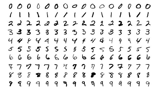
The MNIST dataset
- The MNIST dataset contains 70,000 labeled images of digits, all of which are 28 pixels by 28 pixels and grayscale (no color).
MNIST stands for "Modified National Institute of Standards and Technology". Yann LeCun et. al. are responsible for curating the dataset; read the original webpage for it here.
- The dataset is pre-split into a training set of 60,000 images and test set of 10,000 images.
- Test set performance on MNIST is a common benchmark for evaluating the quality of a classifier.
Convolutional neural networks, one of the most popular model architectures for computer vision, were developed specifically in the context of achieving high accuracy on MNIST.
There are other, similarly-purposed datasets too, like FashionMNIST.
- State of the art neural network-based models have achieved test set accuracies of as high as 99.87%.
See the leaderboard here!
Loading the data
sklearnhas a built-in function for loading datasets from OpenML.
from sklearn.datasets import fetch_openml
X, y = fetch_openml("mnist_784", version=1, return_X_y=True, as_frame=True)
# The documentation here: https://www.openml.org/search?type=data&status=active&id=554
# tells us that the first 60,000 rows constitute the training set.
X_train, X_test = X.iloc[:60000], X.iloc[60000:]
y_train, y_test = y.iloc[:60000].astype(int), y.iloc[60000:].astype(int)
- What do
X_trainandy_trainactually look like?
X_train
| pixel1 | pixel2 | pixel3 | pixel4 | ... | pixel781 | pixel782 | pixel783 | pixel784 | |
|---|---|---|---|---|---|---|---|---|---|
| 0 | 0 | 0 | 0 | 0 | ... | 0 | 0 | 0 | 0 |
| 1 | 0 | 0 | 0 | 0 | ... | 0 | 0 | 0 | 0 |
| 2 | 0 | 0 | 0 | 0 | ... | 0 | 0 | 0 | 0 |
| ... | ... | ... | ... | ... | ... | ... | ... | ... | ... |
| 59997 | 0 | 0 | 0 | 0 | ... | 0 | 0 | 0 | 0 |
| 59998 | 0 | 0 | 0 | 0 | ... | 0 | 0 | 0 | 0 |
| 59999 | 0 | 0 | 0 | 0 | ... | 0 | 0 | 0 | 0 |
60000 rows × 784 columns
y_train
0 5
1 0
2 4
..
59997 5
59998 6
59999 8
Name: class, Length: 60000, dtype: int64
From vectors to images
- In
X_train, each image is represented by a $28 \cdot 28 = 784$-dimensional vector, representing a flattened version of the image.
X_train.iloc[98]
pixel1 0
pixel2 0
pixel3 0
..
pixel782 0
pixel783 0
pixel784 0
Name: 98, Length: 784, dtype: int64
- The first 28 pixels are the first row of the image, the second 28 pixels are the second row of the image, and so on. To view the image, we can reshape the vector into a 2D grid.
X_train.iloc[98].to_numpy().reshape((28, 28))
array([[0, 0, 0, ..., 0, 0, 0],
[0, 0, 0, ..., 0, 0, 0],
[0, 0, 0, ..., 0, 0, 0],
...,
[0, 0, 0, ..., 0, 0, 0],
[0, 0, 0, ..., 0, 0, 0],
[0, 0, 0, ..., 0, 0, 0]])
- Each pixel is represented with a value from 0 to 255, where larger values are more intense (darker in the plot below).
# We'll keep using image 98 as an example, so remember that it's a 3!
util.show_image(X_train.iloc[98])
The distribution of the training set
- Before training any models, we should assess whether there's any class imbalance in the training set.
Remember, we shouldn't peek at the test set until we've actually trained a model.
y_train.value_counts(normalize=True).sort_index().plot(kind='bar', title='Distribution of Digits in the Training Set')
- The 10 possible digits seem to appear at roughly the same frequency.
Model #1: $k$-Nearest Neighbors 🏡🏠
- We can use $k$-nearest neighbors to predict the digit in a new image, $\vec{x}_\text{new} \in \mathbb{R}^{784}$.
Intuitively, this means finding the $k$ "most similar" images to $\vec{x}_\text{new}$.
Remember, $k$-nearest neighbors is a classification method for supervised learning.
- Since we're treating each image in our training set as a "flat" vector in $\mathbb{R}^{784}$, we're ignoring any spatial patterns in each image.
from sklearn.neighbors import KNeighborsClassifier
model_knn = KNeighborsClassifier(n_neighbors=100) # Arbitrary choice; remember, there are 60,000 points in the training set.
model_knn.fit(X_train, y_train)
KNeighborsClassifier(n_neighbors=100)In a Jupyter environment, please rerun this cell to show the HTML representation or trust the notebook.
On GitHub, the HTML representation is unable to render, please try loading this page with nbviewer.org.
KNeighborsClassifier(n_neighbors=100)
- Note that "training" a $k$-NN classifier (i.e. calling
fit) is instant, because nearest neighbor models do all of their calculation upon callingpredict.
- Calling
predictis much slower than callingfit– for each input topredict, the model must find the distance between the input vector and all 60,000 vectors in the training set to see which $k=100$ are the closest.
model_knn.predict(X_train.iloc[[98]])
array([3])
# Accuracy on test set. Takes ~10 seconds on my computer, but is fairly high.
y_test_pred = model_knn.predict(X_test)
(y_test == y_test_pred).mean()
0.944
What kinds of errors does the model make?
- A 100-nearest neighbor classifier achieves 94.4% test set accuracy.
- To further understand the classifier's performance, we can draw its confusion matrix.
X_test_labeled = X_test.assign(
true=y_test,
pred=y_test_pred
)
util.show_confusion(y_test, y_test_pred, title='Confusion Matrix for 100-Nearest Neighbors Model')
- Some of the most common errors seem to be:
- Predicting 1 when the true digit is 2 or 7.
- Predicting 7 when the true digit is 2.
- Predicting 9 when the true digit is 4 or 7.
- Let's peek at some of those cases!
Examining misclassified images
- Run the cell below repeatedly to see a randomly-chosen image from the test set that we classified incorrectly.
util.show_image_and_label(X_test_labeled.query('pred != true').sample().iloc[0])
- Run the cell below repeatedly to see a randomly-chosen image from the test set that we incorrectly classified as a 1.
util.show_image_and_label(X_test_labeled.query('pred != true and pred == 1').sample().iloc[0])
Question 🤔 (Answer at practicaldsc.org/q)
Remember that you can always ask questions anonymously at the link above!
Downsides of $k$-nearest neighbors
- In the example below, our 100-nearest neighbor classifier predicted 1, when the true label was 2.
util.show_image_and_label(X_test_labeled.query('pred != true and pred == 1').iloc[1])
- One downside: $k$-nearest neighbors doesn't incorporate any probability in its decision-making process.
What if we could get a probability that the above image is of a 0, 1, 2, 3, ..., 9?
- Another downside: Classifying a new image takes relatively long.
What if we could learn patterns from the training set in advance, so that predicting new images is relatively quick?
Model #2: Multinomial logistic regression 📈
- Multinomial logistic regression, or softmax regression, predicts the probability that an image $\vec x_i \in \mathbb{R}^{784}$ belongs to each class.
- To train a multinomial logistic regression model for this task, we'll ultimately need to find 10 optimal parameter vectors, $\vec w_0^*$, $\vec w_1^*$, ..., $\vec w_9^*$.
Multinomial logistic regression in sklearn
- As we've seen before, the
LogisticRegressionclass supports multinomial logistic regression.
from sklearn.linear_model import LogisticRegression
model_log = LogisticRegression(multi_class='multinomial', penalty='l1', solver='saga')
model_log
LogisticRegression(multi_class='multinomial', penalty='l1', solver='saga')In a Jupyter environment, please rerun this cell to show the HTML representation or trust the notebook.
On GitHub, the HTML representation is unable to render, please try loading this page with nbviewer.org.
LogisticRegression(multi_class='multinomial', penalty='l1', solver='saga')
- Given that we have 60,000 training examples, each of which are 784-dimensional, training on the full training set takes quite a while – longer than we have time to run in lecture! Just to demonstrate, we'll fit on just the first 10,000 rows of the training set.
model_log.fit(X_train.head(10000), y_train.head(10000))
LogisticRegression(multi_class='multinomial', penalty='l1', solver='saga')In a Jupyter environment, please rerun this cell to show the HTML representation or trust the notebook.
On GitHub, the HTML representation is unable to render, please try loading this page with nbviewer.org.
LogisticRegression(multi_class='multinomial', penalty='l1', solver='saga')
- While calling
fittakes a while, callingpredictis fast.
util.show_image(X_train.iloc[[98]])
model_log.predict(X_train.iloc[[98]])
array([3])
# MUCH faster than with the k-nearest neighbors model.
model_log.score(X_test, y_test)
0.9011
What kinds of errors does this model make?
- The our multinomial logistic regression model, trained on just the first 10,000 rows of the training set, achieves 90.12% test set accuracy.
- Let's peek at the confusion matrix once again.
X_test_labeled = X_test.assign(
true=y_test,
pred=model_log.predict(X_test)
)
util.show_confusion(y_test, model_log.predict(X_test), title='Confusion Matrix for Multinomial Logistic Regression Model')
- The most common types of errors are now different! Common errors:
- Predicting 8 when the true digit is a 2 or 5.
- Predicting 3 when the true digit is a 5 (or vice versa).
Modeling uncertainty
- Let's look at test set images that the multinomial logistic regression model misclassified.
util.show_image_and_label(X_test_labeled.query('pred != true and pred == 8').iloc[15])
- We can use
predict_probato see the distribution of predicted probabilities per class.
model_log.predict_proba(X_test_labeled.query('pred != true and pred == 8').iloc[[15], :-2])
array([[0. , 0. , 0.44, 0.02, 0. , 0. , 0. , 0. , 0.54, 0. ]])
util.visualize_probs(model_log.predict_proba(X_test_labeled.query('pred != true and pred == 8').iloc[[15], :-2]))
Other close calls
- Repeatedly run the cell below to look at the distribution of predicted probabilities for misclassified examples.
t = X_test_labeled.query('pred != true').reset_index(drop=True)
t = t.assign(second_highest_prob = pd.DataFrame(model_log.predict_proba(t.iloc[:, :-2])).apply(lambda r: r.sort_values().iloc[-2], axis=1))
p = t[t['second_highest_prob'] >= 0.3].sample().iloc[0]
util.show_image_and_label(p.iloc[:-1].astype(int)).show()
util.visualize_probs(model_log.predict_proba(p.iloc[:-3].to_frame().T))
Visualizing coefficients
- Since there are 10 classes,
model_loghas 10 parameter vectors (each in $\mathbb{R}^{784}$) – one per class.
model_log.coef_
array([[0., 0., 0., ..., 0., 0., 0.],
[0., 0., 0., ..., 0., 0., 0.],
[0., 0., 0., ..., 0., 0., 0.],
...,
[0., 0., 0., ..., 0., 0., 0.],
[0., 0., 0., ..., 0., 0., 0.],
[0., 0., 0., ..., 0., 0., 0.]])
model_log.coef_.shape
(10, 784)
- We can visualize these coefficients, too!
Below, pixels in blue had a positive coefficient, i.e. increase the probability of class 0. Pixels in red had a negative coefficient, i.e. decrease the probability of class 0.
px.imshow(model_log.coef_[0].reshape((28, 28)), color_continuous_scale='Rdbu', title='Class 0 Coefficients')
util.plot_model_coefficients(model_log.coef_)
Question 🤔 (Answer at practicaldsc.org/q)
Remember that you can always ask questions anonymously at the link above!
Reflection
- We've fit two models to the MNIST training set so far:
- $k$-nearest neighbors.
- Multinomial logistic regression.
- Both models achieved a test set accuracy above 90%.
- Both models are slow in some sense:
- $k$-nearest neighbors is slow at classifying new images.
- Multinomial logistic regression is slow to train.
- These issues, in part, stem from the fact that our design matrix has $28 \cdot 28 = 784$ columns, i.e. 784 features:
X_train
| pixel1 | pixel2 | pixel3 | pixel4 | ... | pixel781 | pixel782 | pixel783 | pixel784 | |
|---|---|---|---|---|---|---|---|---|---|
| 0 | 0 | 0 | 0 | 0 | ... | 0 | 0 | 0 | 0 |
| 1 | 0 | 0 | 0 | 0 | ... | 0 | 0 | 0 | 0 |
| 2 | 0 | 0 | 0 | 0 | ... | 0 | 0 | 0 | 0 |
| ... | ... | ... | ... | ... | ... | ... | ... | ... | ... |
| 59997 | 0 | 0 | 0 | 0 | ... | 0 | 0 | 0 | 0 |
| 59998 | 0 | 0 | 0 | 0 | ... | 0 | 0 | 0 | 0 |
| 59999 | 0 | 0 | 0 | 0 | ... | 0 | 0 | 0 | 0 |
60000 rows × 784 columns
- Is there a way we could reduce the number of features we use, i.e. reduce the number of columns in the design matrix, and still achieve decent test set performance?
Principal component analysis (PCA)
- Principal component analysis (PCA) is an unsupervised learning technique used for dimensionality reduction.
- It'll allow us to take:
X_train, which has 60,000 rows and 784 columns, and transform it intoX_train_approx, which has 60,000 rows and $p$ columns, where $p$ is as small as we want (e.g. $p = 2$).
It creates $p$ new features, each of which is a linear combination of all existing 784 features.
$$\text{new feature 1} = 0.05 \cdot \text{pixel 1} + 0.93 \cdot \text{pixel 2} + ... - \: 0.35 \cdot \text{pixel 784}$$
$$\text{new feature 2} = - 0.06 \cdot \text{pixel 1} + 0.5 \cdot \text{pixel 2} + ... + \: 0.04 \cdot \text{pixel 784}$$
$$...$$
These new features are chosen to capture as much variability (information) in the original data as possible.
- How? The details are out of scope for us, but it leverages the singular value decomposition from linear algebra:
PCA in sklearn
sklearnhas an implementation of PCA, which operates like a transformer.
Remember, PCA is an unsupervised technique! We don't use the actual digit labels for each image when computing this transformation.
from sklearn.decomposition import PCA
pca = PCA(n_components=2)
pca.fit(X_train)
PCA(n_components=2)In a Jupyter environment, please rerun this cell to show the HTML representation or trust the notebook.
On GitHub, the HTML representation is unable to render, please try loading this page with nbviewer.org.
PCA(n_components=2)
- Once
fit,pcacan transformX_traininto a 2-column matrix in a way that retains the bulk of the information:
X_train_approx = pca.transform(X_train)
X_train_approx.shape
(60000, 2)
X_train_approx
array([[ 123.93, 312.67],
[1011.72, 294.86],
[ -51.85, -392.17],
...,
[-178.05, -160.08],
[ 130.61, 5.59],
[-173.44, 24.72]])
- When each data point was 784-dimensional, we couldn't visualize our training set.
But now, each data point is 2-dimensional, which we can easily visualize with a scatter plot!
Visualizing principal components
- The new features that PCA creates are called principal components (PCs).
Note that the principal component values no longer correspond to pixel intensities, which used to range between 0 and 255.
- Plotting PC 2 vs. PC 1 doesn't lead to a ton of insight:
util.show_2_pcs(X_train_approx, y_train)
Clusters in principal components
- But what if we color each point by its true class?
util.show_2_pcs(X_train_approx, y_train, color=True)
- Key idea: Even when projected onto just two principal components, the 0s tend to look alike, the 1s tend to look alike, and so on!
- This doesn't always happen when using PCA; use it as part of your exploratory data analysis toolkit.
PCA as a preprocessing step
- We can use PCA as part of a larger modeling pipeline. We've chosen a number of principal components to use in advance, but in practice we should cross-validate.
from sklearn.pipeline import make_pipeline
model_pca_log = make_pipeline(
PCA(n_components=30),
LogisticRegression(multi_class='multinomial', penalty='l1', solver='saga')
)
model_pca_log
Pipeline(steps=[('pca', PCA(n_components=30)),
('logisticregression',
LogisticRegression(multi_class='multinomial', penalty='l1',
solver='saga'))])In a Jupyter environment, please rerun this cell to show the HTML representation or trust the notebook. On GitHub, the HTML representation is unable to render, please try loading this page with nbviewer.org.
Pipeline(steps=[('pca', PCA(n_components=30)),
('logisticregression',
LogisticRegression(multi_class='multinomial', penalty='l1',
solver='saga'))])PCA(n_components=30)
LogisticRegression(multi_class='multinomial', penalty='l1', solver='saga')
- The transformed data is of a much lower dimension than the raw data. As a result, we can train – and predict – on the full training set very quickly!
model_pca_log.fit(X_train, y_train)
Pipeline(steps=[('pca', PCA(n_components=30)),
('logisticregression',
LogisticRegression(multi_class='multinomial', penalty='l1',
solver='saga'))])In a Jupyter environment, please rerun this cell to show the HTML representation or trust the notebook. On GitHub, the HTML representation is unable to render, please try loading this page with nbviewer.org.
Pipeline(steps=[('pca', PCA(n_components=30)),
('logisticregression',
LogisticRegression(multi_class='multinomial', penalty='l1',
solver='saga'))])PCA(n_components=30)
LogisticRegression(multi_class='multinomial', penalty='l1', solver='saga')
- And the test set accuracy is still good!
model_pca_log.score(X_test, y_test)
0.8869
Parting thoughts 👋
You've accomplished a lot!
- You learned a lot this semester – you're now among the most qualified data scientists in the world!
- You're now able to start with raw data and come up with accurate, meaningful insights that you can share with others.
- You know how to use industry-standard data manipulation tools, and you understand the inner-workings of complicated machine learning models.
- You're well-prepared for internships and data science interviews, ready to create your own portfolio of personal projects, and have the background and maturity to succeed in more advanced data science-adjacent courses.
- Data science is a relatively new, rapidly evolving field, so you'll need to keep evolving with it.
- The tools of the trade may change, but the core principles won't – fortunately, you now have a strong foundation on which you can develop new skills.

My freshman year transcript.
Thank you, and keep in touch!
- Thank you for signing up for this brand-new class!
- The course would not have been possible without our IA, Abhinav, and grader, Angela, who did a lot of work behind the scenes to keep the class running.
- Don't be a stranger – our contact information is at practicaldsc.org/staff. We want to hear about what you do after this class.
This semester's course website will remain online permanently at practicaldsc.org/sp25, so you can refer back to the content.