# Run this cell to get everything set up.
from lec_utils import *
import lec22_util as util
diabetes = pd.read_csv('data/diabetes.csv')
from sklearn.model_selection import train_test_split
diabetes = diabetes[(diabetes['Glucose'] > 0) & (diabetes['BMI'] > 0)]
X_train, X_test, y_train, y_test = (
    train_test_split(diabetes[['Glucose', 'BMI']], diabetes['Outcome'], random_state=1)
)

Lecture 22

Logistic Regression

EECS 398: Practical Data Science, Spring 2025

practicaldsc.org • github.com/practicaldsc/sp25 • 📣 See latest announcements here on Ed

Agenda 📆

• Predicting probabilities.
• Cross-entropy loss.
• From probabilities to decisions.

Check out this Decision Boundary Visualizer, which allows you to visualize decision boundaries for different classifiers.

Question 🤔 (Answer at practicaldsc.org/q)

Remember that you can always ask questions anonymously at the link above!

Predicting probabilities 🎲

---

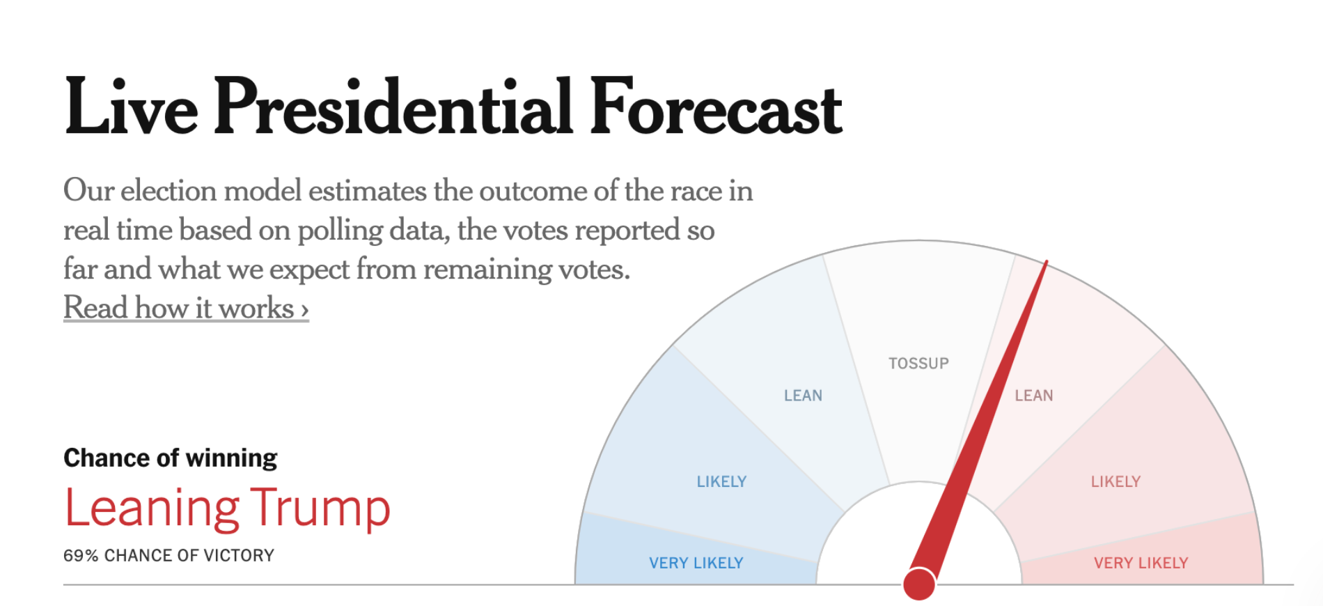
The New York Times maintained needles
that displayed the probabilities of various outcomes in the election.

Motivation: Predicting probabilities

• Often, we're interested in predicting the probability of an event occurring, given some other information.

Given that the score at the start of the second half is Michigan 23-Northwestern 15,
what's the probability that Michigan wins?

Here's a picture of an animal. What's the probability it's of a dog? Cat? Hamster? Zebra?

What's the probability that it rains on campus tomorrow?
In the context of weather apps, this is a nuanced question; here's a meme about it.

• If we're able to predict the probability of an event, we can classify the event by using a threshold.
  For example, if we predict there's a 70% chance of Michigan winning, we could predict that Michigan will win. Here, we implicitly used a threshold of 50%.

• The two classification techniques we've seen so far – $k$-nearest neighbors and decision trees – don't directly use probabilities in their decision-making process.
  But sometimes it's helpful to model uncertainty and to be able to state a level of confidence along with a prediction!

Recap: Predicting diabetes

• As before, class 0 (orange) is "no diabetes" and class 1 (blue) is "diabetes".

util.create_base_scatter(X_train, y_train)

• Let's try to predict whether or not a patient has diabetes ('Outcome') given just their 'Glucose' level.
  Last class, we used both 'Glucose' and 'BMI'; we'll start with just one feature for now.

util.show_one_feature_plot(X_train, y_train)

• It seems that as a patient's 'Glucose' value increases, the chances they have diabetes also increases.

• Can we model this probability directly, as a function of 'Glucose'?
  In other words, can we find some $f$ such that:

$$P(y_i = 1 | \text{Glucose}_i) = f(\text{Glucose}_i)$$

An attempt to predict probabilities

• Let's try and fit a simple linear model to the data from the previous slide.

util.show_one_feature_plot_with_linear_model(X_train, y_train)

• The simple linear model above predicts values greater than 1 and less than 0! This means we can't interpret the outputs as probabilities.

• We could, technically, clip the outputs of the linear model:

util.show_one_feature_plot_with_linear_model_clipped(X_train, y_train)

Bins and proportions

• Another approach we could try is to:
  • Place 'Glucose' values into bins, e.g. 50 to 55, 55 to 60, 60 to 65, etc.
  • Within each bin, compute the proportion of patients in the training set who had diabetes.

# Take a look at the source code in lec22_util.py to see how we did this!
# We've hidden a lot of the plotting code in the notebook to make it cleaner.
util.make_prop_plot(X_train, y_train)

• For example, the point near a 'Glucose' value of 100 has a $y$-axis value of ~0.25. This means that about 25% of patients with a 'Glucose' value near 100 had diabetes in the training set.

• So, if a new person comes along with a 'Glucose' value near 100, we'd predict there's a 25% chance they have diabetes (so they likely do not)!

• Notice that the points form an S-shaped curve!
  Can we incorporate this S-shaped curve in how we predict probabilities?

The logistic function

• The logistic function resembles an $S$-shape.

  $$\sigma(t) = \frac{1}{1 + e^{-t}} = \frac{1}{1 + \text{exp}(-t)}$$

  
  The logistic function is an example of a sigmoid function, which is the general term for an S-shaped function. Sometimes, we use the terms "logistic function" and "sigmoid function" interchangeably.

• Below, we'll look at the shape of $y = \sigma(w_0 + w_1 x)$ for different values of $w_0$ and $w_1$.
  • $w_0$ controls the position of the curve on the $x$-axis.
  • $w_1$ controls the "steepness" of the curve.

util.show_three_sigmoids()

• Notice that $0 < \sigma(t) < 1$, for all $t$, which means we can interpret the outputs of $\sigma(t)$ as probabilities!

Below, interact with the sliders to change the values of $w_0$ and $w_1$.

interact(util.plot_sigmoid, w0=(-15, 15), w1=(-3, 3, 0.1));

interactive(children=(IntSlider(value=0, description='w0', max=15, min=-15), FloatSlider(value=0.0, descriptio…

Logistic regression

• Logistic regression is a linear classification technique that builds upon linear regression.
  It is not called logistical regression!

• It models the probability of belonging to class 1, given a feature vector:

$$P(y_i = 1 | \vec{x}_i) = \sigma (\underbrace{w_0 + w_1 x_i^{(1)} + w_2 x_i^{(2)} + ... + w_d x_i^{(d)}}_{\text{linear regression model}}) = \sigma\left(\vec{w} \cdot \text{Aug}(\vec{x}_i) \right)$$

• Note that the existence of coefficients, $w_0, w_1, ... w_d$, that we need to learn from the data, tells us that logistic regression is a parametric method!

LogisticRegression in sklearn

from sklearn.linear_model import LogisticRegression

• Let's fit a LogisticRegression classifier. Specifically, this means we're asking sklearn to learn the optimal parameters $w_0^*$ and $w_1^*$ in:

$$P(y_i = 1 | \text{Glucose}_i) = \sigma \left( w_0 + w_1 \cdot \text{Glucose}_i \right)$$

model_logistic = LogisticRegression()
model_logistic.fit(X_train[['Glucose']], y_train)

LogisticRegression()

In a Jupyter environment, please rerun this cell to show the HTML representation or trust the notebook.
On GitHub, the HTML representation is unable to render, please try loading this page with nbviewer.org.

• We get a test accuracy that's roughly in line with the test accuracies of the two models we saw last class.

model_logistic.score(X_test[['Glucose']], y_test)

0.75

• What does our fit model look like?

Visualizing a fit logistic regression model

• The values of $w_0^*$ and $w_1^*$ sklearn found are below.

model_logistic.intercept_[0], model_logistic.coef_[0][0]

(-5.594502656264591, 0.039958336242438434)

• So, our fit model is:

$$P(y_i = 1 | \text{Glucose}_i) = \sigma(-5.59 + 0.04 \cdot \text{Glucose}_i)$$

util.show_one_feature_plot_with_logistic(X_train, y_train)

• So, if a patient has a 'Glucose' level of 150, the model's predicted probability that they have diabetes is:

$$\sigma(-5.59 + 0.04 \cdot 150) \approx \sigma(0.41) \approx 0.601$$

model_logistic.predict_proba([[150]])

array([[0.4, 0.6]])

How did sklearn find $w_0^*$ and $w_1^*$?
What loss function did it use?

Cross-entropy loss

---

The modeling recipe

• To train a parametric model, we always follow the same three steps.

$k$-Nearest Neighbors and decision trees didn't quite follow the same process.

1. Choose a model.

$$P(y_i = 1 | \vec{x}_i) = \sigma (w_0 + w_1 x_i^{(1)} + w_2 x_i^{(2)} + ... + w_d x_i^{(d)}) = \sigma\left(\vec{w} \cdot \text{Aug}(\vec{x}_i) \right)$$

2. Choose a loss function.

???

3. Minimize average loss to find optimal model parameters.
   As we've now seen, average loss could also be regularized!

???

Attempting to use squared loss

• Our default loss function has always been squared loss, so we could try and use it here.

$$R_\text{sq}(\vec{w}) = \frac{1}{n} \sum_{i = 1}^n \left( y_i - \sigma\left(\vec{w} \cdot \text{Aug}(\vec{x}_i) \right) \right)^2$$

• Unfortunately, there's no closed form solution for $\vec{w}^*$, so we'll need to use gradient descent.

• Before doing so, let's visualize the loss surface in the case of our "simple" logistic model:

$$P(y_i = 1 | \text{Glucose}_i) = \sigma(w_0 + w_1 \cdot \text{Glucose}_i)$$

• Specifically, we'll visualize:

$$R_\text{sq}(w_0, w_1) = \frac{1}{n} \sum_{i = 1}^n \left( y_i - \sigma(w_0 + w_1 \underbrace{x_i}_{\text{Glucose}_i} ) \right)^2$$

util.show_logistic_mse_surface(X_train, y_train)