from lec_utils import *
import lec20_util as util

Lecture 20

Gradient Descent

EECS 398: Practical Data Science, Winter 2025

practicaldsc.org • github.com/practicaldsc/wn25 • 📣 See latest announcements here on Ed

Agenda 📆

• Intuition for gradient descent 🗻.
• When is gradient descent guaranteed to work?
• Gradient descent for functions of multiple variables.

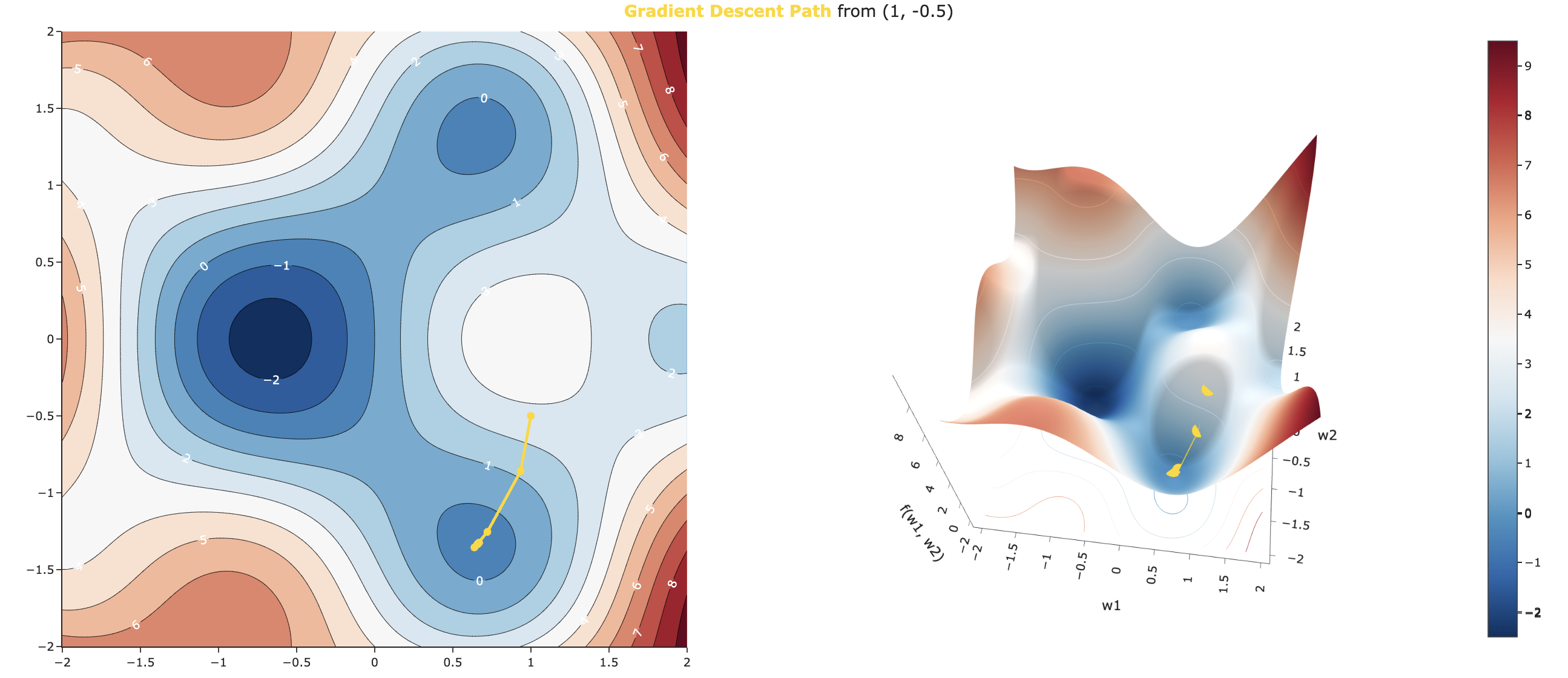
What we're building towards today.

Question 🤔 (Answer at practicaldsc.org/q)

Remember that you can always ask questions anonymously at the link above!

Intuition for gradient descent 🗻

---

Let's go hiking!

• Suppose you're at the top of a mountain 🏔️ and need to get to the bottom.

• Further, suppose it's really cloudy ☁️, meaning you can only see a few feet around you.

• How would you get to the bottom?

Minimizing arbitrary functions

• Assume $f(w)$ is some differentiable function.
  For now, we'll assume $f$ takes in a scalar, $w$, as input and returns a scalar as its output.

• When tasked with minimizing $f(w)$, our general strategy has been to:
  
  1. Find $\frac{df}{dw}(w)$, the derivative of $f$.
  2. Find the input $w^*$ such that $\frac{df}{dw}(w^*) = 0$.

• However, there are cases where we can find $\frac{df}{dw}(w)$, but it is either difficult or impossible to solve $\frac{df}{dw}(w^*) = 0$. Then what?

$$f(w) = 5w^4 - w^3 - 5w^2 + 2w - 9$$

util.draw_f()

What does the derivative of a function tell us?

• Goal: Given a differentiable function $f(w)$, find the input $w^*$ that minimizes $f(w)$.

• What does $\frac{d}{dw} f(w)$ mean?

from ipywidgets import interact
interact(util.show_tangent, w0=(-1.5, 1.5));

interactive(children=(FloatSlider(value=0.0, description='w0', max=1.5, min=-1.5), Output()), _dom_classes=('w…

Searching for the minimum

• Suppose we're given an initial guess for a value of $w$ that minimizes $f(w)$.

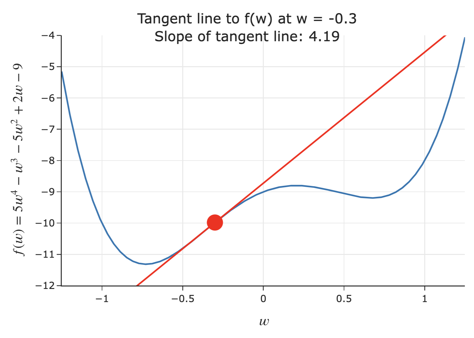
• If the slope of the tangent line at $f(w)$ is positive 📈:
  • Increasing $w$ increases $f$.
  • This means the minimum must be to the left of the point $(w, f(w))$.
  • Solution: Decrease $w$ ⬇️.

• The steeper the slope is, the further we must be from the minimum – so, the steeper the slope, the quicker we should decrease $w$!

Searching for the minimum

• Suppose we're given an initial guess for a value of $w$ that minimizes $f(w)$.

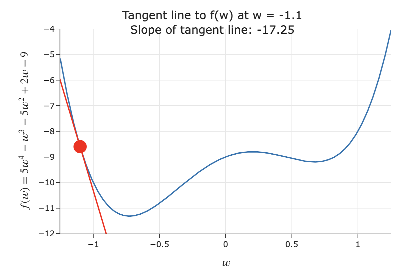
• If the slope of the tangent line at $f(w)$ is negative 📉:
  • Increasing $w$ decreases $f$.
  • This means the minimum must be to the right of the point $(w, f(w))$.
  • Solution: Increase $w$ ⬆️.

• The steeper the slope is, the further we must be from the minimum – so, the steeper the slope, the quicker we should increase $w$!

Gradient descent

• To minimize a differentiable function $f$:
  1. Pick a positive number, $\alpha$. This number is called the learning rate, or step size.
     Think of $\alpha$ as a hyperparameter of the minimization process.
  2. Pick an initial guess, $w^{(0)}$.
  3. Then, repeatedly update your guess using the update rule:

$$w^{(t+1)} = w^{(t)} - \alpha \frac{df}{dw}(w^{(t)})$$

• Repeat this process until convergence – that is, when the difference between $w^{(t)}$ and $w^{(t+1)}$ is small.

• This procedure is called gradient descent.

What is gradient descent?

• Gradient descent is a numerical method for finding the input to a function $f$ that minimizes the function.

• It is called gradient descent because the gradient is the extension of the derivative to functions of multiple variables.

• A numerical method is a technique for approximating the solution to a mathematical problem, often by using the computer.

• Gradient descent is widely used in machine learning, to train models from linear regression to neural networks and transformers (including ChatGPT)!
  In machine learning, we use gradient descent to minimize empirical risk when we can't minimize it by hand, which is true in most, more sophisticated cases.

Implementing gradient descent

• In practice, we typically don't implement gradient descent ourselves – we rely on existing implementations of it. But, we'll implement it here ourselves to understand what's going on.

• Let's start with an initial guess $w^{(0)} = 0$ and a learning rate $\alpha = 0.01$.

$$w^{(t+1)} = w^{(t)} - \alpha \frac{df}{dw}(w^{(t)})$$

w = 0
for t in range(50):
    print(round(w, 4), round(util.f(w), 4))
    w = w - 0.01 * util.df(w)

0 -9
-0.02 -9.042
-0.042 -9.0927
-0.0661 -9.1537
-0.0925 -9.2267
-0.1214 -9.3135
-0.1527 -9.4158
-0.1866 -9.5347
-0.2229 -9.6708
-0.2615 -9.8235
-0.302 -9.9909
-0.344 -10.1687
-0.3867 -10.3513
-0.4293 -10.5311
-0.4709 -10.7001
-0.5104 -10.8511
-0.547 -10.9789
-0.58 -11.0811
-0.6089 -11.1586
-0.6335 -11.2141
-0.654 -11.2521
-0.6706 -11.277
-0.6839 -11.2927
-0.6943 -11.3023
-0.7023 -11.308
-0.7085 -11.3113
-0.7131 -11.3132
-0.7166 -11.3143
-0.7193 -11.3149
-0.7213 -11.3153
-0.7227 -11.3155
-0.7238 -11.3156
-0.7247 -11.3156
-0.7253 -11.3157
-0.7257 -11.3157
-0.726 -11.3157
-0.7263 -11.3157
-0.7265 -11.3157
-0.7266 -11.3157
-0.7267 -11.3157
-0.7268 -11.3157
-0.7268 -11.3157
-0.7269 -11.3157
-0.7269 -11.3157
-0.7269 -11.3157
-0.7269 -11.3157
-0.727 -11.3157
-0.727 -11.3157
-0.727 -11.3157
-0.727 -11.3157

• We see that pretty quickly, $w^{(t)}$ converges to $-0.727$!

Visualizing $w^{(0)} = 0, \alpha = 0.01$

util.minimizing_animation(w0=0, alpha=0.01)

Visualizing $w^{(0)} = 1.1, \alpha = 0.01$

What if we start with a different initial guess?

util.minimizing_animation(w0=1.1, alpha=0.01)

Visualizing $w^{(0)} = 0, \alpha = 0.1$

What if we use a different learning rate?

util.minimizing_animation(w0=0, alpha=0.1)

Visualizing $w^{(0)} = 0, \alpha = 1$

Some learning rates are so large that the values of $w$ explode towards infinity! Watch what happens when we use a learning rate of 1:

w = 0
for t in range(50):
    print(round(w, 4), round(util.f(w), 4))
    w = w - 1 * util.df(w)

0 -9
-2 55
148 2395575055
-64768502 87988399093209215258221002525055
5434024027622804955958648 4359696148872124725882822307832767315039587443442298737093378524825544745642834622818997783401350055
-3209184300040232968384986400955563373214898401121991075501068665288470367002 530332985231284587741390981348980358147931180953380132783007883732290450487940896497686801834821479793056750838217464306331399631782539963635649924968096560953483216630744135148611918314690619239216181828228590993041527070916340763511348214767483482898617989266963488210286317855470338346244530924050055
661019044901392416954729679460748990344170910956358835698132854563403750799535254895720517200327333237179123918683068293585779703016725909751539139711861617687813209841593304288472547260824104926792650829880677991116888105447148 954609811130853181103583701649028211653660744627023839503556744987120626567103558567559598665702180831022338880115370491802698434832577366874991589662088965037117816221504923258001678540709754551409196622983402075423897917311140276279241141570865352818912580292076157317652459623227622008267704418865451565124850508363893736669815765725665667366255955451825529239205112277975621646590805843102421929101874916034353375181650823160240275221716639504237816856330637620915336423852170198623085839171048441345753566891271423134343990416913972889069267978119649974190469814710715636873538491644959256191689099590275341151171819790272788767702188985877934107603998669287604787308015484964644983093480091708331796112794087571003132797188774464919854845084662160823258121712229906414297355334067702069889036890811444360852930909406532971705798565032317088519403066294374222935955758358426585115485869844584732865071125055
-5776594901426824677760480474882267759584323573334469245518728218477211441849170261086790265427887646502160199028651631032865248664657546774385277227975572113996889604118144335449979370344701318004957758483337360534957311016716528158918733168768987913212630157201130190714745075686287645254078551834810276130815287367029241908776773753955285997149825750202626302129245121512515240250913385951208276563237429345711741762020109539150320627994866580511418312312651021359018659779452045853422296670672741295547252935058529308187027533149563829451002796785142110224887498329653640450635931265679232291798563741794599235612163962019705986436274936065651608305243446437666621321660450426195502 5567467040762316647385680347496459071251908329594160637160498217500728208197785446877620158646539654196693804349701586885505176356827181880839354738173998718197881791881967695457924075375294149630473701323151168952512549575023461459967449672579482008885831745929142141307525902417921966422620156197997959033382481547789109206030074643294774657208648370969358486991923314222057795753918515226937876476501703483528201605196470687213979945800918422889559476532497715529745247540647183908990046566458091964430977720304527045774223725630445826305008926134177414636165239732270281548434945740006290454894345971654799317870476761859071358456700605388406526672352852842528562812080157563678373872972299765360359661781260039830550782774851103914104460053225713254665083723090034914553217854973947491715388082781371837178415343779041114832420266562516738494930908406864990809290469065201457416742355159387931761288948089880134766558012048604589614427248226611670883138104212484824576364868456607848641544085419408684803182641302222711849442851846688984202685218850146983425835148344713877943139507299503363868320438698755066216665031441301315464067215418012635191464658042702741661722755979820460469677297995810315811215663898912622910102255559762850130312289787292854714575891715793598025092374164364282959494877810669555805022547146134781462745383374343668249780501716400740138568430849172523027689098838759922274029309133123478995142169995505126232505676819213088714715656287738858154533136855634026888245481898579026078615890721196538637229193944104541362086415076437862917954223027414916208781786565842299215444273960692425511146694322624069953293786875830319514711885802415773788409813779243749524914244516213710663260063688335921887369244677554825392081574955007731473426560520821688595689782468311769547938315083428262015533566031818211680185018320653621298397725185879170798176531103648662701549010048950888729070216090647184538768143166154511376277117235807121203111830861246070656539536355204462276388648953881233443527113872654284387900650540683367971947151628154490986163371145377670078048070618732564773855322256383844757843718007771960314271730413963708642094262402184015551513234118077484341995264719171815862502578409011729975998047461884275026017838376240794591113391051148546757147128595410875481466482193442309330997235009212240046797730355829181690992079997293491670138092017754077150230363231768901357800214696847752712490141376479743191489292002260894100178579654600753149959455619099748751239885506374502836267293906056062286685319228208301660012222246228506117164074258953811501120138459015981704650114720296390762242471158059548639639927387729533173665405132394910446596550820016373570414868657854973615617172836900954575055
3855189526540728524278319589985944495280538183882299698111689637316917381014217424359204367757696569848797009286892542400785193726335567987034823263801379873053783159408920759828571423350123520123035158696353085032635136034131454305531324732236086118636591592766279126638843826115442262604630257496291581655380520525571414258044875312841352532019938871383343877558513337813374125880178988558766709859899290450137866624221730719608783942726161612792292305504566249374395980642467567218942150593990395152526094519095131463300406217865689511779704428711817280647109327850769428626549065765980036609088275619449954869385676998947910213629191812252524723398626483312884863537692238044139790238208452983272310794434698544113549330856479690021344599732952778985508833957294859477035036071847071599443134882108915531890138690637316504153318235252832248766928560532967615588730273287698123681564030077662024861886093041219973225909975993186676633428845630829511044966800955808789774160870559946654821874915508336277098360788879945103538972629204066467239792918237167786057571888151366709626913042986689083367879892696729560516485898681940815106502563918787990749571977850666555457934714778242970898998055380928540525862898129526293837152588892472464187926016910874594710823808523892486983995786101954775129386224417798737057254745757493815140576352882408891677979092062423913177607696314891502599572041093610228309909244092496865578650805891175698700745462968934690359706927049642045485713846183931306952972003913491311485079791450461936196070640685465196727010011659512276761228081942347860844708394750775631606546197508835071877303456351730912372251498497086485867526328442126596521073598894369578656924259173657522539931993404043814903461522066789523205765659882980970713576706897118147377104743538840122956532911071796144453651876484893964959088019075578216005476795649512420435265088056097629087650340512140436442510445645669612970287029900222069693894940747901277423995624030099301782502790091665044221793488568935328647585524597829056270452373090049303865648 

---------------------------------------------------------------------------
ValueError                                Traceback (most recent call last)
Cell In[8], line 3
      1 w = 0
      2 for t in range(50):
----> 3     print(round(w, 4), round(util.f(w), 4))
      4     w = w - 1 * util.df(w)

ValueError: Exceeds the limit (4300) for integer string conversion; use sys.set_int_max_str_digits() to increase the limit

Lingering questions

• When is gradient descent guaranteed to converge to a global minimum? What kinds of functions work well with gradient descent?

• How do we choose a step size?

• How do we use gradient descent to minimize functions of multiple variables, e.g.:

$$R_\text{ridge}(\vec{w}) = \frac{1}{n} \lVert \vec{y} - X \vec{w} \rVert^2 + \lambda \sum_{j = 1}^d w_j^2$$This is a function of $d+1$ variables: $w_0, w_1, ..., w_d$.

• Question: Why can't we use gradient descent to find $\vec{w}_\text{LASSO}^*$?

$$R_\text{LASSO}(\vec{w}) = \frac{1}{n} \lVert \vec{y} - X \vec{w} \rVert^2 + \lambda \sum_{j = 1}^d |w_d|$$

When is gradient descent guaranteed to work?

---

What makes a function convex?

A convex function ✅.

A non-convex function ❌.

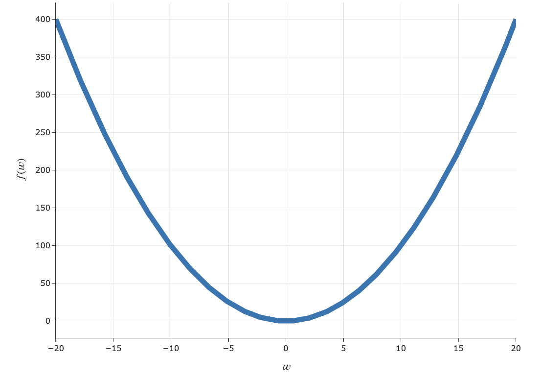
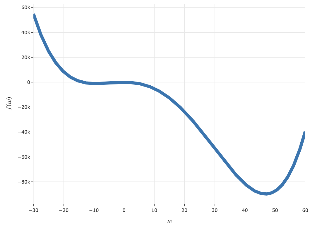
Intuitive definition of convexity

A convex function ✅.

A non-convex function ❌.

• A function $f$ is convex if, for every $a, b$ in the domain of $f$, the line segment between:

  $$(a, f(a)) \text{ and } (b, f(b))$$

  does not go below the plot of $f$.

• See the reference slides for the formal definition.

Reference Slide

Formal definition of convexity

• A function $f: \mathbb{R} \rightarrow \mathbb{R}$ is convex if, for every $a, b$ in the domain of $f$, and for every $t \in [0, 1]$:

$$\boxed{(1 - t) f(a) + t f(b) \geq f((1-t)a + tb)}$$

• This is a formal way of restating the definition from the previous slide.

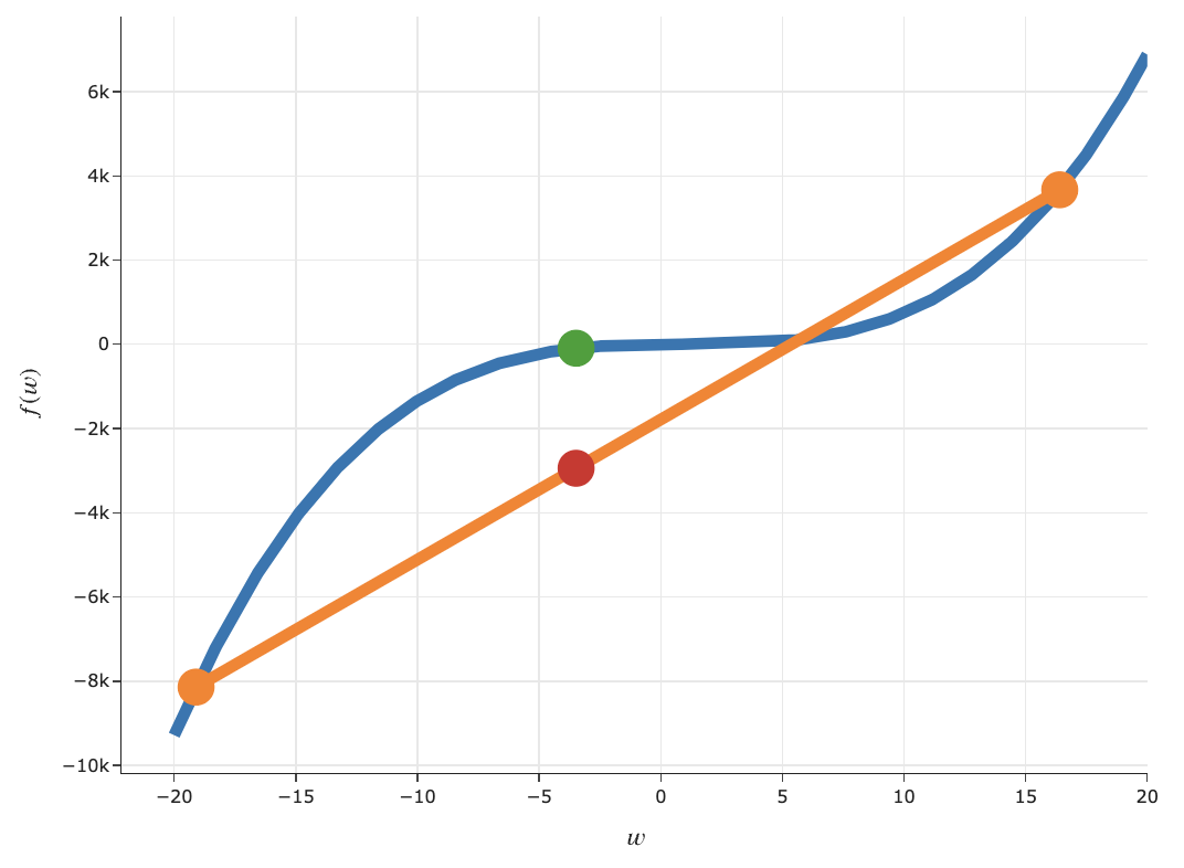
• The slider below depicts an interactive version of the formal definition of convexity above.
  Drag the a, b, and t sliders and see what happens!

interact(util.convexity_visual, a=(-20, 5, 0.1), b=(5, 20, 0.1), t=FloatSlider(min=0, max=1, step=0.01, value=0.5));

interactive(children=(FloatSlider(value=-8.0, description='a', max=5.0, min=-20.0), FloatSlider(value=12.0, de…

Second derivative test for convexity

• If $f(w)$ is a function of a single variable and is twice differentiable, then $f(w)$ is convex if and only if:

$$\frac{d^2f}{dw^2}(w) \geq 0, \:\:\: \forall \: w$$

• Example: $f(w) = w^4$ is convex.

Why does convexity matter?

• Convex functions are (relatively) easy to minimize with gradient descent.

• Theorem: If $f(w)$ is convex and differentiable, then gradient descent converges to a global minimum of $f$, as long as the step size is small enough.

• Why?
  • Gradient descent converges when the derivative is 0.
  • For convex functions, the derivative is 0 only at one place – the global minimum.
  • In other words, if $f$ is convex, gradient descent won't get "stuck" and terminate in places that aren't global minimums (local minimums, saddle points, etc.).

Nonconvex functions and gradient descent

• We say a function is nonconvex if it does not meet the criteria for convexity.

• Nonconvex functions are (relatively) difficult to minimize.

• Gradient descent might still work, but it's not guaranteed to find a global minimum.
  • We saw this at the start of the lecture, when trying to minimize $f(w) = 5w^4 - w^3 - 5w^2 + 2w - 9$.

Choosing a step size in practice

• In practice, choosing a step size involves a lot of trial-and-error.

• In this class, we've only touched on "constant" step sizes, i.e. where $\alpha$ is a constant.

$$w^{(t+1)} = w^{(t)} - \alpha \frac{df}{dw}(w^{(t)})$$

• Remember: $\alpha$ is the "step size", but the amount that our guess for $w$ changes is $\alpha \frac{df}{dw}(w^{(t)})$, not just $\alpha$.

• In future courses, you may learn about "decaying" step sizes, where the value of $\alpha$ decreases as the number of iterations increases.
  Intuition: take much bigger steps at the start, and smaller steps as you progress, as you're likely getting closer to the minimum.

Gradient descent for functions of multiple variables

---

Minimizing functions of multiple variables

• We will typically use gradient descent to minimize empirical risk functions, $R(\vec w)$, to find optimal model parameters.
  A model with $d+1$ parameters $w_0, w_1, ..., w_d$ will have a $(d+2)$-dimensional loss surface.

• Consider the following example function $f: \mathbb{R}^2 \rightarrow \mathbb{R}$:

$$f(w_1, w_2) = 3 \sin(2 w_1) \cos(2 w_2) + w_1^2 + w_2^2$$

util.make_3D_surface()

util.make_3D_contour()

Minimizing functions of multiple variables

• Consider the function:

$$f(w_1, w_2) = 3 \sin(2 w_1) \cos(2 w_2) + w_1^2 + w_2^2$$

• It has two partial derivatives: $\frac{\partial f}{\partial w_1}$ and $\frac{\partial f}{\partial w_2}$.
  See the annotated slides for what they are and how we find them.

The gradient vector

• If $f(\vec{w})$ is a function of multiple variables, then its gradient, $\nabla f (\vec{w})$, is a vector containing its partial derivatives.

• Example:

$$f(\vec{w}) = f(w_1, w_2) = 3 \sin(2 w_1) \cos(2 w_2) + w_1^2 + w_2^2$$$$\nabla f(\vec w) = \begin{bmatrix} 6\cos(2w_1)\cos(2w_2) + 2w_1 \\ -6\sin(2w_1)\sin(2w_2) + 2w_2 \end{bmatrix}$$

• Example:

$$f(\vec{w}) = \vec{w}^T \vec{w}$$$$\nabla f(\vec{w}) = 2 \vec{w}$$

What does the gradient vector describe?

• Consider the visual example from two slides ago.

$$f(\vec{w}) = f(w_1, w_2) = 3 \sin(2 w_1) \cos(2 w_2) + w_1^2 + w_2^2$$$$\nabla f(\vec w) = \begin{bmatrix} 6\cos(2w_1)\cos(2w_2) + 2w_1 \\ -6\sin(2w_1)\sin(2w_2) + 2w_2 \end{bmatrix}$$

util.make_3D_contour(with_gradient=True, w1_start=-0.2, w2_start=0.5)

• The gradient vector at a point ($w_1, w_2$) describes the direction of steepest ascent, i.e. the direction in which the function $f$ is increasing the quickest, when standing at $(w_1, w_2)$.

Moving against the gradient

• The gradient vector at a point ($w_1, w_2$) describes the direction of steepest ascent, i.e. the direction in which the function $f$ is increasing the quickest, when standing at $(w_1, w_2)$.

• To minimize $f$, when starting at ($w_1, w_2$), we should move in the direction opposite to the gradient!

util.make_3D_contour(with_gradient=True, w1_start=-0.2, w2_start=0.5, neg=True)

Gradient descent for functions of multiple variables

• Example:

$$f(\vec{w}) = f(w_1, w_2) = 3 \sin(2 w_1) \cos(2 w_2) + w_1^2 + w_2^2$$$$\nabla f(\vec w) = \begin{bmatrix} 6\cos(2w_1)\cos(2w_2) + 2w_1 \\ -6\sin(2w_1)\sin(2w_2) + 2w_2 \end{bmatrix}$$

• The global minimizer* of $f$ is a vector, $\vec{w}^* = \begin{bmatrix} w_1^* \\ w_2^* \end{bmatrix}$.
  *If one exists.

• We start with an initial guess, $\vec{w}^{(0)}$, and step size $\alpha$, and update our guesses using:

$$\vec{w}^{(t+1)} = \vec{w}^{(t)} - \alpha \nabla f(\vec{w}^{(t)})$$

Gradient descent for functions of multiple variables

• Let's visualize the execution of gradient descent on our trigonometric example.
  Change w1_start, w2_start, and step_size below and see what happens!

util.display_paths(w1_start=1, w2_start=-0.5, iterations=10, step_size=0.1)

Activity

Consider the following function.

$$f(w_1, w_2) = (w_1-2)^2 + 2w_1 - (w_2-3)^2$$

Given an initial guess of $\vec{w}^{(0)} = \begin{bmatrix} 0 \\ 0 \end{bmatrix}$ and a step size of $\alpha = \frac{1}{3}$, perform two iterations of gradient descent. What is $\vec{w}^{(2)}$?

Example: Gradient descent for simple linear regression

• To find optimal model parameters for the model $H(x_i) = w_0 + w_1 x_i$ and squared loss, we minimized empirical risk:

$$R_\text{sq}(w_0, w_1) = R_\text{sq}(\vec{w}) = \frac{1}{n} \sum_{i = 1}^n ( y_i - (w_0 + w_1 x_i ))^2$$

• This is a function of multiple variables, and is differentiable, so it has a gradient!

$$\nabla R(\vec{w}) = \begin{bmatrix} \displaystyle -\frac{2}{n} \sum_{i = 1}^n (y_i - (w_0 + w_1 x_i)) \\ \displaystyle -\frac{2}{n} \sum_{i = 1}^n (y_i - (w_0 + w_1x_i))x_i \end{bmatrix}$$

• Key idea: To find $\vec{w}^* = \begin{bmatrix} w_0^* \\ w_1^* \end{bmatrix}$, we could use gradient descent!

• Why would we, when closed-form solutions exist?

Gradient descent for simple linear regression, visualized

YouTubeVideo('oMk6sP7hrbk')

Gradient descent for simple linear regression, implemented

• Let's use gradient descent to fit a simple linear regression model to predict commute time in 'minutes' from 'departure_hour'.

df = pd.read_csv('data/commute-times.csv')
df[['departure_hour', 'minutes']]

util.make_scatter(df)

x = df['departure_hour']
y = df['minutes']

• First, let's remind ourselves what $w_0^*$ and $w_1^*$ are supposed to be.

slope = np.corrcoef(x, y)[0, 1] * np.std(y) / np.std(x)
slope

-8.186941724265557

intercept = np.mean(y) - slope * np.mean(x)
intercept

142.44824158772875

Implementing partial derivatives

$$R_\text{sq}(\vec{w}) = \frac{1}{n} \sum_{i = 1}^n ( y_i - (w_0 + w_1 x_i ))^2$$$$\nabla R(\vec{w}) = \begin{bmatrix} \displaystyle -\frac{2}{n} \sum_{i = 1}^n (y_i - (w_0 + w_1 x_i)) \\ \displaystyle -\frac{2}{n} \sum_{i = 1}^n (y_i - (w_0 + w_1x_i))x_i \end{bmatrix}$$

def dR_w0(w0, w1):
    return -2 * np.mean(y - (w0 + w1 * x))

def dR_w1(w0, w1):
    return -2 * np.mean((y - (w0 + w1 * x)) * x)

Implementing gradient descent

• The update rule we'll follow is:

$$\vec{w}^{(t+1)} = \vec{w}^{(t)} - \alpha \nabla R(\vec{w}^{(t)})$$

• We can treat this as two separate update equations:

$$w_0^{(t+1)} = w_0^{(t)} - \alpha \frac{\partial R}{\partial w_0} (\vec{w}^{(t)}) \\ w_1^{(t+1)} = w_1^{(t)} - \alpha \frac{\partial R}{\partial w_1} (\vec{w}^{(t)})$$

• Let's initialize $w_0^{(0)} = 100$ and $w_1^{(0)} = -50$, and choose the step size $\alpha = 0.01$.
  The initial guesses were just parameters that we thought might be close.

# We'll store our guesses so far, so we can look at them later.
def gradient_descent_for_regression(w0_initial, w1_initial, alpha, threshold=0.0001):
    w0, w1 = w0_initial, w1_initial
    
    w0_history = [w0]
    w1_history = [w1]

    while True:
        w0 = w0 - alpha * dR_w0(w0, w1)
        w1 = w1 - alpha * dR_w1(w0, w1)

        w0_history.append(w0)
        w1_history.append(w1)
        
        if np.abs(w0_history[-1] - w0_history[-2]) <= threshold:
            break
    
    return w0_history, w1_history

w0_history, w1_history = gradient_descent_for_regression(0, 0, 0.01)

w0_history[-1]

142.1051891023626

w1_history[-1]

-8.146983792459055

• It seems that we converge at the right value! But how many iterations did it take? What could we do to speed it up?

len(w0_history)

20664