from lec_utils import *
import lec19_util as util
from IPython.display import Markdown
from sklearn.linear_model import LinearRegression
from sklearn.preprocessing import PolynomialFeatures, OneHotEncoder, FunctionTransformer, StandardScaler
from sklearn.model_selection import train_test_split, GridSearchCV
from sklearn.pipeline import make_pipeline
from sklearn.compose import make_column_transformer

Lecture 19

Regularization

EECS 398: Practical Data Science, Winter 2025

practicaldsc.org • github.com/practicaldsc/wn25 • 📣 See latest announcements here on Ed

Agenda 📆

• Recap: Model selection.
• Ridge regression 🏔️.
• LASSO 📿.

Remember to look at the Machine Learning section of the Resources tab of the course website.

In addition, this lecture has an associated Guide, which we'll refer to in lecture and you'll need to read for Homework 9.

Question 🤔 (Answer at practicaldsc.org/q)

Remember that you can always ask questions anonymously at the link above!

Recap: Model selection

---

Example: Commute times

• Last class, we used $k$-fold cross-validation to choose between the following five models that predict commute time in 'minutes'.

• Which model has the highest model bias?
  See the annotated slides for the answer.

• Which model has the highest model variance?

• Which model is most likely to perform best in practice? Why?

Ridge regression 🏔️

---

Motivation

• So far, to us, "model complexity" has essentially meant "number of features."
  The main hyperparameter we've tuned is polynomial degree. For instance, a polynomial of degree 5 has 5 features – an $x$, $x^2$, $x^3$, $x^4$, and $x^5$ feature.
  In the more recent example, we manually created several different pipelines, each of which used different combinations of features from the commute times dataset.

• Once we've created several different candidate models, we've used cross-validation to choose the one that best generalizes to unseen data.

• Another approach: instead of manually choosing which features to include, put some constraint on the optimal parameters, $w_0^*, w_1^*, ..., w_d^*$.
  This would save us time from having to think of combinations of features that might be relevant.

• Intuition: The bigger the optimal parameters $w_0^*, w_1^*, ..., w_d^*$ are, the more overfit the model is to the training data.
  Why?

Polynomial regression returns

• Last class, we fit various polynomial regression models to Sample 1, shown below.

sample_1 = util.sample_from_pop()
X_train, X_test, y_train, y_test = train_test_split(sample_1[['x']], sample_1['y'], random_state=23)
px.scatter(x=X_train['x'], y=y_train, title="Sample 1's Training Data", width=800, height=600)

• As we increase the degree of the polynomial, the resulting fit polynomial overfits the training data more and more.

interact(lambda d: util.fit_and_show_fit(X_train, y_train, d)[1], d=(1, 25));

Inspecting the fit degree 25 polynomial

• Let's consider the degree 25 polynomial.

model, fig = util.fit_and_show_fit(X_train, y_train, d=25)
fig

• What does the fit polynomial actually look like, as an equation?

# These coefficients are rounded to two decimal places.
# The coefficient on x^25 is not 0.00, but is something very small.
util.display_features(model.named_steps['linearregression'])

$$0.07+13.20x-3.43x^{2}-184.70x^{3}+137.47x^{4}+737.22x^{5}-652.75x^{6}-1383.99x^{7}+1408.31x^{8}+1406.82x^{9}-1722.03x^{10}-760.88x^{11}+1286.70x^{12}+147.59x^{13}-599.20x^{14}+62.28x^{15}+169.59x^{16}-47.32x^{17}-26.14x^{18}+12.69x^{19}+1.26x^{20}-1.59x^{21}+0.17x^{22}+0.07x^{23}-0.02x^{24}+0.00x^{25}$$

util.plot_coefficient_magnitudes(model.named_steps['linearregression'])

• sklearn assigned really large coefficients to many features.
  This means that if $x$ changes a little, the output is going to change a lot. It seems like some of the terms are trying to "cancel" each other out – some have large negative coefficients, some have large positive coefficients.

• Intuition: In general, the larger the optimal parameters $w_0^*, w_1^*, ..., w_d^*$ are, the more overfit the model is to the training data.

Ridge regression

• Idea: In addition to just minimizing mean squared error, what if we could also try and prevent large parameter values?
  Maybe this would lead to less overfitting!

• Regularization is the act of adding a penalty on the norm of the parameter vector, $\vec w$, to the objective function.

$$R_\text{ridge}(\vec{w}) = \frac{1}{n} \lVert \vec{y} - X \vec{w} \rVert^2 \:\: + \underbrace{\lambda \sum_{j = 1}^d w_j^2}_{{\substack{\text{regularization} \\ \text{penalty}}}}$$

• Linear regression with $L_2$ regularization – as shown above – is called ridge regression.
  You'll explore the reason why in Homework 9!

• Intuition: Instead of just minimizing mean squared error, we balance minimizing mean squared error and a penalty on the size of the fit coefficients, $w_1^*$, $w_2^*$, ..., $w_d^*$.
  We don't regularize the intercept term!

• $\lambda$ is a hyperparameter, which we choose through cross-validation.

• The $\vec{w}_\text{ridge}^*$ that minimizes $R_\text{ridge}(\vec{w})$ is not necessarily the same as $\vec{w}_\text{OLS}^*$, which minimizes $R_\text{sq}(\vec{w})$!

Activity

The objective function we minimize to find $\vec{w}_\text{ridge}^*$ in ridge regression is:

$$R_\text{ridge}(\vec{w}) = \frac{1}{n} \lVert \vec{y} - X \vec{w} \rVert^2 + \lambda \sum_{j = 1}^d w_j^2$$

$\lambda$ is a hyperparameter, which we choose through cross-validation. Discuss the following points with those near you:

• What if we pick $\lambda = 0$ – what is $\vec{w}_\text{ridge}^*$ then?
• What happens to $\vec{w}_\text{ridge}^*$ as $\lambda \rightarrow \infty$?
• Can $\lambda$ be negative?

Another interpretation of ridge regression

• As $\lambda$ increases, the penalty on the size of $\vec{w}_\text{ridge}^*$ increases, meaning that each $w_j^*$ inches closer to 0.

• An equivalent way of formulating the ridge regression objective function,

  $$\text{minimize} \:\:\:\: \frac{1}{n} \lVert \vec{y} - X \vec{w} \rVert^2 + \lambda \sum_{j = 1}^d w_j^2$$

  is as a constrained optimization problem:

  $$\text{minimize} \:\:\:\:\frac{1}{n} \lVert \vec{y} - X \vec{w} \rVert^2 \text{ such that } \sum_{j = 1}^d w_j^2 \leq Q$$

• $Q$ and $\lambda$ are inversely related: the larger $Q$ is, the less of a penalty we're putting on size of $\vec{w}_\text{ridge}^*$, so the smaller $\lambda$ is.

  $$\lambda \approx \frac{1}{Q}$$

  
  The exact relationship between $Q$ and $\lambda$ is outside of the scope of this course, as is the proof of this fact.

Aside: Contour plots

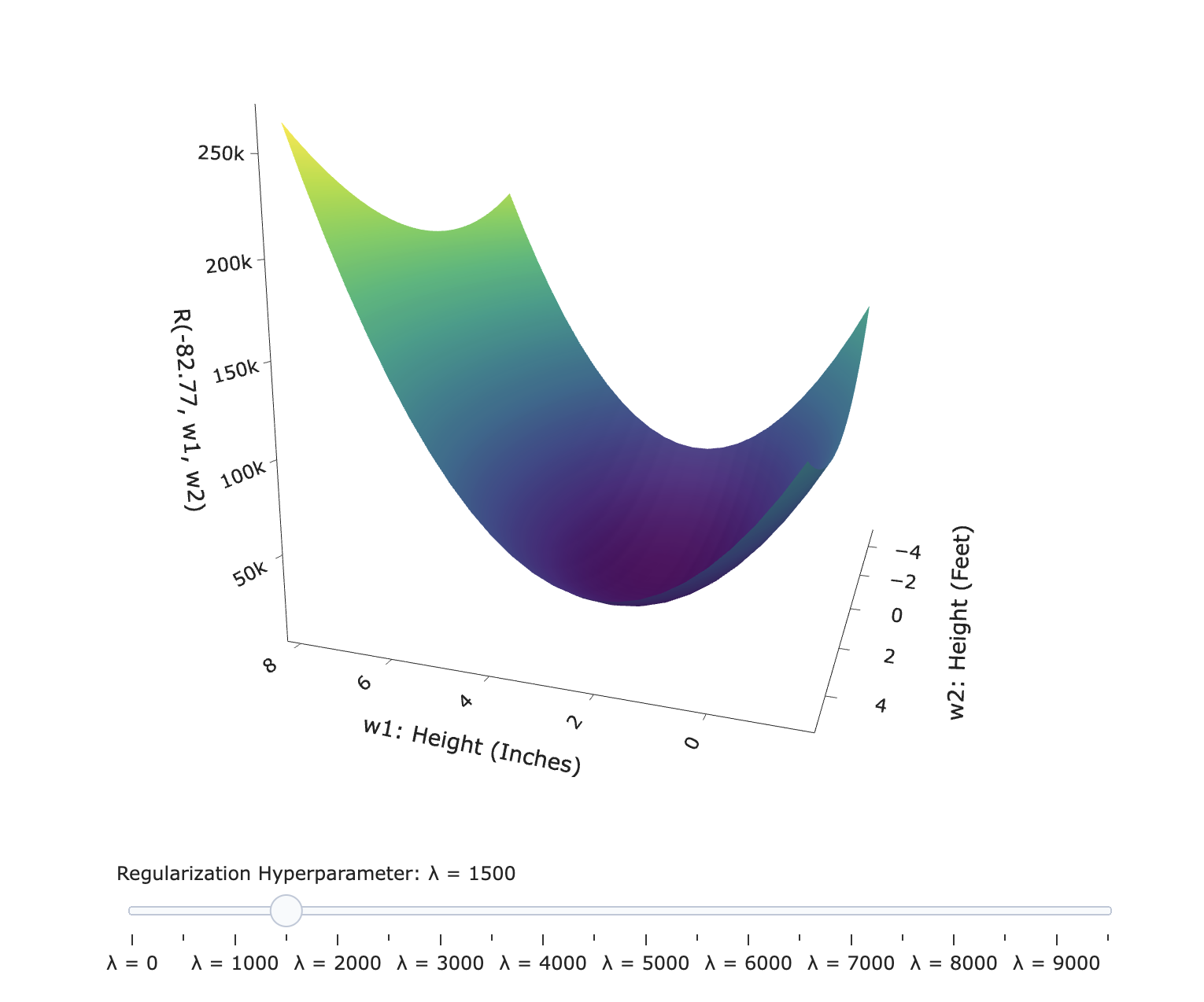
• First, let's look at the loss surface for mean squared error without regularization, for some two feature regression model.

util.show_ols_surface()

• We can equivalently visualize this 3D surface as a contour plot, which can be thought of as a projection of the surface above into two dimensions, with the colors preserved.
  Learn more about contour plots in this video.

util.show_ols_contour()

Visualizing ridge regression as a constrained optimization problem

$$\text{minimize} \:\:\:\:\frac{1}{n} \lVert \vec{y} - X \vec{w} \rVert^2 \text{ such that } \sum_{j = 1}^d w_j^2 \leq Q; \qquad \lambda \approx \frac{1}{Q}$$

• Intuitively:

  • The contour plot of the loss surface for just the mean squared error component is in viridis.
  • The constraint, $\sum_{j = 1}^d w_j^2 \leq Q$, is in red. Ridge regression says, minimize mean squared error, while staying in the red circle.
    The larger $Q$ is, the larger the radius of the circle is.

util.show_ridge_contour()

• The smaller $Q$ is – so, the larger $\lambda$ is – the smaller the red circle is!

• As $\lambda$ increases, the constrained solution $\vec w_\text{ridge}^*$ shrinks closer to $\vec 0$.

Finding $\vec{w}_\text{ridge}^*$

• We know that the $\vec{w}_\text{OLS}^*$ that minimizes mean squared error, $$R_\text{sq}(\vec{w}) = \frac{1}{n} \lVert \vec{y} - X \vec{w} \rVert^2$$ is the one that satisfies the normal equations, $X^TX \vec{w} = X^T \vec{y}$.
  Recall, linear regression that minimizes mean squared error, without any other constraints, is called ordinary least squares (OLS).

• Sometimes, $\vec{w}^*_\text{OLS}$ is unique, and sometimes there are infinitely many possible $\vec{w}^*_\text{OLS}$.
  There are infinitely many possible $\vec{w}^*_\text{OLS}$ when the design matrix, $X$, is not full rank! All of these infinitely many solutions minimize mean squared error.

• Which vector $\vec{w}_\text{ridge}^*$ minimizes the ridge regression objective function?

$$R_\text{ridge}(\vec{w}) = \frac{1}{n} \lVert \vec{y} - X \vec{w} \rVert^2 + \lambda \sum_{j = 1}^d w_j^2$$

• It turns out there is always a unique solution for $\vec{w}_\text{ridge}^*$, even if $X$ is not full rank. It is: $$\vec{w}_\text{ridge}^* = (X^TX + n \lambda I)^{-1} X^T \vec{y}$$
  You'll prove this in Homework 9!

• Since there is always a unique solution, ridge regression is often used in the presence of multicollinearity!

Visualizing ridge regression as an unconstrained optimization problem

• In the new Ridge Regression guide, we dive deeper into some of the theory of ridge regression.

• Scroll to the section titled Loss surfaces to see an interactive visualization on the effect of $\lambda$ on the shape of the objective function's loss surface:

$$R_\text{ridge}(\vec{w}) = \frac{1}{n} \lVert \vec{y} - X \vec{w} \rVert^2 + \lambda \sum_{j = 1}^d w_j^2$$

Taking a step back

• $\vec{w}_\text{ridge}^*$ doesn't minimize mean squared error – it minimizes a slightly different objective function.

• So, why would we use ever use ridge regression?

Ridge regression in sklearn

• Fortunately, sklearn can perform ridge regression for us.

from sklearn.linear_model import Ridge

• Just to experiment, let's set $\lambda$ to something extremely large and look at the resulting predictions.

# The name of the lambda hyperparameter in sklearn is alpha.
model_large_lambda = make_pipeline(PolynomialFeatures(25, include_bias=False), 
                                   Ridge(alpha=1000000000000000000000000000))
model_large_lambda.fit(X_train, y_train)

Pipeline(steps=[('polynomialfeatures',
                 PolynomialFeatures(degree=25, include_bias=False)),
                ('ridge', Ridge(alpha=1000000000000000000000000000))])

In a Jupyter environment, please rerun this cell to show the HTML representation or trust the notebook.
On GitHub, the HTML representation is unable to render, please try loading this page with nbviewer.org.

Visualizing the extremely regularized model

• What do the resulting predictions look like?

util.plot_given_model_dict(X_train, y_train, {'Extremely Regularized Polynomial of Degree 25': (model_large_lambda, 'purple')})

• What do you notice?

model_large_lambda.named_steps['ridge'].intercept_

3.6606542664388497

# All 0!
model_large_lambda.named_steps['ridge'].coef_

array([0., 0., 0., ..., 0., 0., 0.])

y_train.mean()

3.662415381952351

Using GridSearchCV to choose $\lambda$

• In general, we won't just arbitrarily choose a value of $\lambda$.

• Instead, we'll perform $k$-fold cross-validation to choose the $\lambda$ that leads to predictions that work best on unseen test data.
  The value of $\lambda$ depends on the specific dataset and model you've chosen; there's no universally "best" $\lambda$.

hyperparams = {
    'ridge__alpha': 10.0 ** np.arange(-2, 15) # Try 0.01, 0.1, 1, 10, 100, 1000, ... 
}
model_regularized = GridSearchCV(
    estimator=make_pipeline(PolynomialFeatures(25, include_bias=False), Ridge()),
    param_grid=hyperparams,
    scoring='neg_mean_squared_error'
)
model_regularized.fit(X_train, y_train)

GridSearchCV(estimator=Pipeline(steps=[('polynomialfeatures',
                                        PolynomialFeatures(degree=25,
                                                           include_bias=False)),
                                       ('ridge', Ridge())]),
             param_grid={'ridge__alpha': array([1.e-02, 1.e-01, 1.e+00, 1.e+01, 1.e+02, 1.e+03, 1.e+04, 1.e+05,
       1.e+06, 1.e+07, 1.e+08, 1.e+09, 1.e+10, 1.e+11, 1.e+12, 1.e+13,
       1.e+14])},
             scoring='neg_mean_squared_error')

In a Jupyter environment, please rerun this cell to show the HTML representation or trust the notebook.
On GitHub, the HTML representation is unable to render, please try loading this page with nbviewer.org.

• Let's check the optimal $\lambda$ it found!

model_regularized.best_params_

{'ridge__alpha': 1000000000.0}

• While we used GridSearchCV here, note that RidgeCV also exists, which performs automatic cross-validation.

Visualizing the regularized degree 25 model

• What do the resulting predictions look like?

util.plot_given_model_dict(X_train, y_train,
                           {'Unregularized Polynomial of Degree 25': (model, '#ff7f0f'),
                            'Regularized Polynomial of Degree 25': (model_regularized, 'green')})

• It seems that the regularized polynomial is less overfit to the specific noise in the training data than the unregularized polynomial!

• The largest coefficients are all much smaller now, too.

The coefficient on $x^{20}$ is -0.000136.

util.display_features(model_regularized.best_estimator_.named_steps['ridge'], precision=8)

$$0.53107052+0.00000013x+0.00000003x^{2}+0.00000031x^{3}+0.00000014x^{4}+0.00000081x^{5}+0.00000053x^{6}+0.00000221x^{7}+0.00000181x^{8}+0.00000615x^{9}+0.00000566x^{10}+0.00001655x^{11}+0.00001569x^{12}+0.00004094x^{13}+0.00003602x^{14}+0.00008574x^{15}+0.00005684x^{16}+0.00012909x^{17}+0.00001744x^{18}+0.00008493x^{19}-0.00013594x^{20}-0.00000611x^{21}+0.00003794x^{22}-0.00000702x^{23}-0.00000154x^{24}+0.00000037x^{25}$$

util.plot_coefficient_magnitudes(model_regularized.best_estimator_.named_steps['ridge'])

• Note that none of them are exactly 0, but many of them are close!
  This will be important later.

Tuning multiple hyperparameters at once

• What if we don't want to fix a polynomial degree in advance, and instead want to choose both the degree and value of $\lambda$ using cross-validation?

• No problem – we can still grid search.
  Note that the next cell takes much longer than the previous call to fit took, since it needs to try every combination of $\lambda$ and polynomial degree.

hyperparams = {
    'ridge__alpha': 10.0 ** np.arange(-2, 15),
    'polynomialfeatures__degree': range(1, 26)
}
model_regularized_degree = GridSearchCV(
    estimator=make_pipeline(PolynomialFeatures(include_bias=False), Ridge()),
    param_grid=hyperparams,
    scoring='neg_mean_squared_error'
)
model_regularized_degree.fit(X_train, y_train)

GridSearchCV(estimator=Pipeline(steps=[('polynomialfeatures',
                                        PolynomialFeatures(include_bias=False)),
                                       ('ridge', Ridge())]),
             param_grid={'polynomialfeatures__degree': range(1, 26),
                         'ridge__alpha': array([1.e-02, 1.e-01, 1.e+00, 1.e+01, 1.e+02, 1.e+03, 1.e+04, 1.e+05,
       1.e+06, 1.e+07, 1.e+08, 1.e+09, 1.e+10, 1.e+11, 1.e+12, 1.e+13,
       1.e+14])},
             scoring='neg_mean_squared_error')

In a Jupyter environment, please rerun this cell to show the HTML representation or trust the notebook.
On GitHub, the HTML representation is unable to render, please try loading this page with nbviewer.org.

• Now, let's check the optimal $\lambda$ and polynomial degree it found!

model_regularized_degree.best_params_

{'polynomialfeatures__degree': 3, 'ridge__alpha': 100.0}

Visualizing the regularized degree 3 model

• What do the resulting predictions look like?

polyfig = util.plot_given_model_dict(X_train, y_train,
                                     {'Unregularized Polynomial of Degree 25': (model, '#ff7f0f'),
                                      'Regularized Polynomial of Degree 25': (model_regularized, 'green'),
                                      'Regularized Polynomial of Degree 3': (model_regularized_degree, 'skyblue')})
polyfig

util.display_features(model_regularized_degree.best_estimator_.named_steps['ridge'])

$$0.21+0.28x+0.04x^{2}+0.97x^{3}$$

Run the cell below to set up the next slide.

from sklearn.metrics import mean_squared_error
unregularized_train = mean_squared_error(y_train, model.predict(X_train))
unregularized_test = mean_squared_error(y_test, model.predict(X_test))
regularized_lambda_train = mean_squared_error(y_train, model_regularized.predict(X_train))
regularized_lambda_validation = (-model_regularized.cv_results_['mean_test_score']).min()
regularized_lambda_test = mean_squared_error(y_test, model_regularized.predict(X_test))
regularized_lambda_degree_train = mean_squared_error(y_train, model_regularized_degree.predict(X_train))
regularized_lambda_degree_validation = (-model_regularized_degree.cv_results_['mean_test_score']).min()
regularized_lambda_degree_test = mean_squared_error(y_test, model_regularized_degree.predict(X_test))
results_df = pd.DataFrame(index=['training MSE', 'average validation MSE (across all folds)', 'test MSE']).assign(
    unregularized=[unregularized_train, np.nan, unregularized_test],
    regularized_lambda_only=[regularized_lambda_train, regularized_lambda_validation, regularized_lambda_test],
    regularized_lambda_and_degree=[regularized_lambda_degree_train, regularized_lambda_degree_validation, regularized_lambda_degree_test]
)

reprs = {'unregularized': '<b><span style="color:#ff7f0f">Unregularized (Degree 25)</span></b>',
         'regularized_lambda_only': '<b><span style="color:green">Regularized (Degree 25)<br><small>Used cross-validation to choose $\lambda$</span></b>',
         'regularized_lambda_and_degree': '<b><span style="color:skyblue">Regularized (Degree 3)<br><small>Used cross-validation to choose $\lambda$ and degree</small></span></b>'}

results_df_str = results_df.to_html()
for rep in reprs:
    results_df_str = results_df_str.replace(rep, reprs[rep])

Comparing training, validation, and test errors

• Let's compare the training and testing error of the three polynomials below.

polyfig

display(HTML(results_df_str))

	Unregularized (Degree 25)	Regularized (Degree 25) Used cross-validation to choose $\lambda$	Regularized (Degree 3) Used cross-validation to choose $\lambda$ and degree
training MSE	4.72	10.33	7.11
average validation MSE (across all folds)	NaN	17.60	7.40
test MSE	14.21	17.17	10.52

• It seems that the regularized polynomial, in which we used cross-validation to choose both the regularization penalty $\lambda$ and degree, generalizes best to unseen data.

What's next?

• Could we have chosen a different method of penalizing each $w_j$ other than $w_j^2$?
  We're about to see another option!

• Ridge regression's objective function happened to have a closed-form solution.
  What if we want to minimize a function that can't be minimized by hand?
  We'll talk about how in the next lecture!

Question 🤔 (Answer at practicaldsc.org/q)

What questions do you have about ridge regression?

LASSO 📿

---

Penalizing large parameters

• The ridge regression objective function, $$R_\text{ridge}(\vec{w}) = \frac{1}{n} \lVert \vec{y} - X \vec{w} \rVert^2 + \lambda \sum_{j = 1}^d w_j^2$$ minimizes mean squared error, plus a squared penalty on the size of the fit coefficients, $w_1^*, w_2^*, ..., w_d^*$.

• Could we have regularized, or penalized the coefficients, in some other way?

• The LASSO objective function penalizes the absolute value of each coefficient:

  $$R_\text{LASSO}(\vec{w}) = \frac{1}{n} \lVert \vec{y} - X \vec{w} \rVert^2 + \lambda \sum_{j = 1}^d |w_j| $$

• LASSO stands for "least absolute shrinkage and selection operator."
  We'll make sense of this name shortly.

Aside: Vector norms

• The $L_2$ norm, or Euclidean norm, of a vector $\vec v \in \mathbb{R}^n$ is defined as:

$$\lVert \vec v \rVert = \lVert \vec v \rVert_2 = \sqrt{v_1^2 + v_2^2 + ... + v_n^2} = \big(v_1^2 + v_2^2 + ... + v_n^2 \big)^\frac{1}{2} $$The $L_2$ norm is the default norm, which is why the subscript 2 is often omitted.

• The $L_p$ norm of $\vec v$, for $p \geq 1$, is:

$$\lVert \vec v \rVert_p = \big(|v_1|^p + |v_2|^p + ... + |v_n|^p \big)^\frac{1}{p}$$

• Ridge regression is said to use $L_2$ regularization because it penalizes the (squared) $L_2$ norm of $\vec w$, ignoring the intercept term:

  $$R_\text{ridge}(\vec{w}) = \frac{1}{n} \lVert \vec{y} - X \vec{w} \rVert^2 + \lambda \sum_{j = 1}^d w_j^2$$

• LASSO is said to use $L_1$ regularization because it penalizes the $L_1$ norm of $\vec w$, ignoring the intercept term:

  $$R_\text{LASSO}(\vec{w}) = \frac{1}{n} \lVert \vec{y} - X \vec{w} \rVert^2 + \lambda \sum_{j = 1}^d |w_j| $$

LASSO in sklearn

• Unlike with ridge regression or ordinary least squares, there is no general closed-form solution for $\vec{w}_\text{LASSO}^*$.

• But, it can be estimated using numerical methods, which sklearn uses under-the-hood. Let's test it out.
  More on numerical methods soon!

from sklearn.linear_model import Lasso

• Let's use LASSO to fit a degree 25 polynomial to Sample 1.
  Here, we'll fix the degree, and cross-validate to find $\lambda$.

hyperparams = {
    'lasso__alpha': 10.0 ** np.arange(-2, 15)
}
model_regularized_lasso = GridSearchCV(
    estimator=make_pipeline(PolynomialFeatures(25, include_bias=False), Lasso()),
    param_grid=hyperparams,
    scoring='neg_mean_squared_error'
)
model_regularized_lasso.fit(X_train, y_train)

GridSearchCV(estimator=Pipeline(steps=[('polynomialfeatures',
                                        PolynomialFeatures(degree=25,
                                                           include_bias=False)),
                                       ('lasso', Lasso())]),
             param_grid={'lasso__alpha': array([1.e-02, 1.e-01, 1.e+00, 1.e+01, 1.e+02, 1.e+03, 1.e+04, 1.e+05,
       1.e+06, 1.e+07, 1.e+08, 1.e+09, 1.e+10, 1.e+11, 1.e+12, 1.e+13,
       1.e+14])},
             scoring='neg_mean_squared_error')

In a Jupyter environment, please rerun this cell to show the HTML representation or trust the notebook.
On GitHub, the HTML representation is unable to render, please try loading this page with nbviewer.org.

• Our cross-validation routine ends up choosing $\lambda = 0.1$, though on its own, this doesn't really tell us anything.

model_regularized_lasso.best_params_

{'lasso__alpha': 0.1}

Visualizing the regularized degree 25 model, fit with LASSO

• What do the resulting predictions look like, relative to the fit polynomials from earlier in the lecture?

util.plot_given_model_dict(X_train, y_train,
                                     {'Unregularized Polynomial of Degree 25': (model, '#ff7f0f'),
                                      'Regularized Polynomial of Degree 25': (model_regularized, 'green'),
                                      'Regularized Polynomial of Degree 3': (model_regularized_degree, 'skyblue'),
                                      'Regularized Polynomial of Degree 25, using LASSO': (model_regularized_lasso, 'red')})

• What do you notice about the coefficients of the polynomial themselves?

util.display_features(model_regularized_lasso.best_estimator_.named_steps['lasso'], precision=8)

$$0.40824893-0.26401764x^{2}+0.99531953x^{3}-0.11522087x^{4}+0.09663804x^{5}+0.03689987x^{6}-0.00932372x^{7}+0.00309213x^{8}-0.00149464x^{9}+0.00014825x^{10}-0.00013611x^{11}+0.00000201x^{12}-0.00001045x^{13}-0.00000032x^{14}-0.00000069x^{15}-0.00000002x^{16}-0.00000003x^{17}$$

• Important: Note that we fit a degree 25 polynomial, but many of the higher-order terms are missing, since their coefficients ended up being exactly 0!
  There's are no $x^{18}, x^{19}, x^{20}, ..., x^{25}$ terms above, and also no $x$ term.

• The resulting polynomial ends up being of degree 17.

When using LASSO, many coefficients are set to 0!

• When using $L_1$ regularization – that is, when performing LASSO – many of the optimal coefficients $w_1^*, w_2^*, ..., w_d^*$ end up being exactly 0.

• This was not the case in ridge regression – there, the optimal coefficients were all very small, but none were exactly 0.

display(Markdown('#### Fit using Ridge:'))
util.display_features(model_regularized.best_estimator_.named_steps['ridge'], precision=8)

Fit using Ridge:

$$0.53107052+0.00000013x+0.00000003x^{2}+0.00000031x^{3}+0.00000014x^{4}+0.00000081x^{5}+0.00000053x^{6}+0.00000221x^{7}+0.00000181x^{8}+0.00000615x^{9}+0.00000566x^{10}+0.00001655x^{11}+0.00001569x^{12}+0.00004094x^{13}+0.00003602x^{14}+0.00008574x^{15}+0.00005684x^{16}+0.00012909x^{17}+0.00001744x^{18}+0.00008493x^{19}-0.00013594x^{20}-0.00000611x^{21}+0.00003794x^{22}-0.00000702x^{23}-0.00000154x^{24}+0.00000037x^{25}$$

util.plot_coefficient_magnitudes(model_regularized.best_estimator_.named_steps['ridge'])

• If a feature has a coefficient of 0, it means it's not being used at all in making predictions.

display(Markdown('#### Fit using LASSO (notice the larger coefficient on $x^3$):'))
util.display_features(model_regularized_lasso.best_estimator_.named_steps['lasso'], precision=8)

Fit using LASSO (notice the larger coefficient on $x^3$):

$$0.40824893-0.26401764x^{2}+0.99531953x^{3}-0.11522087x^{4}+0.09663804x^{5}+0.03689987x^{6}-0.00932372x^{7}+0.00309213x^{8}-0.00149464x^{9}+0.00014825x^{10}-0.00013611x^{11}+0.00000201x^{12}-0.00001045x^{13}-0.00000032x^{14}-0.00000069x^{15}-0.00000002x^{16}-0.00000003x^{17}$$

util.plot_coefficient_magnitudes(model_regularized_lasso.best_estimator_.named_steps['lasso'])

• LASSO implicitly performs feature selection for us – it automatically tells us which features we don't need to use.
  Here, it told us "don't use $x$, don't use $x^{18}$, don't use $x^{19}$, ..., don't use $x^{25}$, and instead weigh the $x^2$ and $x^3$ terms more."

• This is where the name "least absolute shrinkage and selection operator" comes from.

Why does LASSO encourage sparsity?

• The fact that many of the optimal coefficients – $w_1^*, w_2^*, ..., w_d^*$ – are 0 when performing LASSO is often stated as:

LASSO encourages sparsity.

• To make sense of this, let's look at the equivalent formulation of LASSO as a constrained optimization problem.

  $$\text{minimize} \:\:\:\: \frac{1}{n} \lVert \vec{y} - X \vec{w} \rVert^2 + \lambda \sum_{j = 1}^d | w_j |$$

  is equivalent to:

  $$\text{minimize} \:\:\:\:\frac{1}{n} \lVert \vec{y} - X \vec{w} \rVert^2 \text{ such that } \sum_{j = 1}^d | w_j | \leq Q$$

• Again, $Q$ and $\lambda$ are inversely related: the larger $Q$ is, the less of a penalty we're putting on size of $\vec{w}_\text{LASSO}^*$, so the smaller $\lambda$ is.

Visualizing LASSO as a constrained optimization problem

$$\text{minimize} \:\:\:\:\frac{1}{n} \lVert \vec{y} - X \vec{w} \rVert^2 \text{ such that } \sum_{j = 1}^d |w_j| \leq Q; \qquad \lambda \approx \frac{1}{Q}$$

• As before:

  • The contour plot of the loss surface for just the mean squared error component is in viridis.
  • The constraint, $\sum_{j = 1}^d |w_j| \leq Q$, is in red. LASSO says, minimize mean squared error, while staying in the red diamond.
    The larger $Q$ is, the larger the side length of the diamond is.

util.show_lasso_contour()

• Notice that the constraint set has clearly defined "corners," which lie on the axes. The axes are where the parameter values, $w_1$ and $w_2$ here, are 0.

• Due to the shape of the constraint set, it's likely that the minimum value of mean squared error, among all options in the red diamond, will occur at a corner, where some of the parameter values are 0.

Question 🤔 (Answer at practicaldsc.org/q)

What questions do you have about LASSO, or regularization in general?

Example: Commute times

---

Another example: Commute times

• Last class, before we learned about regularization, we used $k$-fold cross-validation to choose between the following five models that predict commute time in 'minutes'.

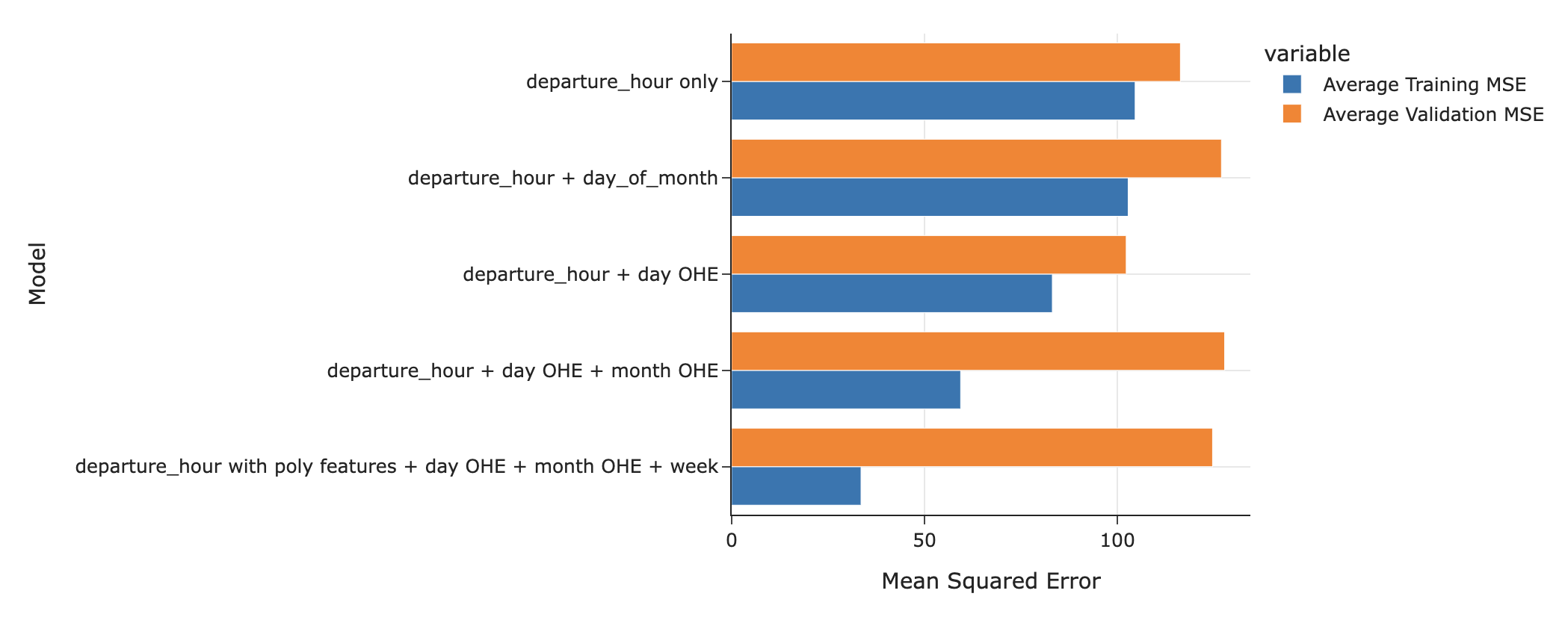
• The most complicated model, labeled departure_hour with poly features + day OHE + month OHE + week, didn't generalize well to unseen data, relative to more simple models.
  At least, not when we used ordinary least squares to train it.

• Let's use ordinary least squares, ridge regression, and LASSO to train the most complicated model from above, and compare the results.

df = pd.read_csv('data/commute-times.csv')
df['day_of_month'] = pd.to_datetime(df['date']).dt.day
df['month'] = pd.to_datetime(df['date']).dt.month_name()
df.head()

	date	day	home_departure_time	home_departure_mileage	...	work_departure_time_hr	mileage_to_home	day_of_month	month
0	5/15/2023	Mon	2023-05-15 10:49:00	15873.0	...	17.17	53.0	15	May
1	5/16/2023	Tue	2023-05-16 07:45:00	15979.0	...	NaN	NaN	16	May
2	5/22/2023	Mon	2023-05-22 08:27:00	50407.0	...	15.90	54.0	22	May
3	5/23/2023	Tue	2023-05-23 07:08:00	50535.0	...	NaN	NaN	23	May
4	5/30/2023	Tue	2023-05-30 09:09:00	50664.0	...	17.12	54.0	30	May

5 rows × 20 columns

X_train, X_test, y_train, y_test = train_test_split(df.drop('minutes', axis=1), df['minutes'], random_state=23)

Ordinary least squares for commute times

• The Pipeline below implements the feature transformations necessary to produce the

  departure_hour with poly features + day OHE + month OHE + week

  model from the last slide.

week_converter = FunctionTransformer(lambda s: 'Week ' + ((s - 1) // 7 + 1).astype(str),
                                     feature_names_out='one-to-one')
day_of_month_transformer = make_pipeline(week_converter, OneHotEncoder(drop='first'))
# Note the include_bias=False once again!
commute_feature_pipe = make_pipeline(
    make_column_transformer(
        (PolynomialFeatures(3, include_bias=False), ['departure_hour']),
        (OneHotEncoder(drop='first', handle_unknown='ignore'), ['day', 'month']),
        (day_of_month_transformer, ['day_of_month']),
    )
)

• First, we'll fit a "vanilla" linear regression model, i.e. one that just minimizes mean squared error, with no regularization.

commute_model_ols = make_pipeline(commute_feature_pipe, LinearRegression())
commute_model_ols

Pipeline(steps=[('pipeline',
                 Pipeline(steps=[('columntransformer',
                                  ColumnTransformer(transformers=[('polynomialfeatures',
                                                                   PolynomialFeatures(degree=3,
                                                                                      include_bias=False),
                                                                   ['departure_hour']),
                                                                  ('onehotencoder',
                                                                   OneHotEncoder(drop='first',
                                                                                 handle_unknown='ignore'),
                                                                   ['day',
                                                                    'month']),
                                                                  ('pipeline',
                                                                   Pipeline(steps=[('functiontransformer',
                                                                                    FunctionTransformer(feature_names_out='one-to-one',
                                                                                                        func=<function <lambda> at 0x16b711fc0>)),
                                                                                   ('onehotencoder',
                                                                                    OneHotEncoder(drop='first'))]),
                                                                   ['day_of_month'])]))])),
                ('linearregression', LinearRegression())])

In a Jupyter environment, please rerun this cell to show the HTML representation or trust the notebook.
On GitHub, the HTML representation is unable to render, please try loading this page with nbviewer.org.

• There are no hyperparameters to grid search for here, so we'll just fit the model directly.

commute_model_ols.fit(X_train, y_train)

Pipeline(steps=[('pipeline',
                 Pipeline(steps=[('columntransformer',
                                  ColumnTransformer(transformers=[('polynomialfeatures',
                                                                   PolynomialFeatures(degree=3,
                                                                                      include_bias=False),
                                                                   ['departure_hour']),
                                                                  ('onehotencoder',
                                                                   OneHotEncoder(drop='first',
                                                                                 handle_unknown='ignore'),
                                                                   ['day',
                                                                    'month']),
                                                                  ('pipeline',
                                                                   Pipeline(steps=[('functiontransformer',
                                                                                    FunctionTransformer(feature_names_out='one-to-one',
                                                                                                        func=<function <lambda> at 0x16b711fc0>)),
                                                                                   ('onehotencoder',
                                                                                    OneHotEncoder(drop='first'))]),
                                                                   ['day_of_month'])]))])),
                ('linearregression', LinearRegression())])

In a Jupyter environment, please rerun this cell to show the HTML representation or trust the notebook.
On GitHub, the HTML representation is unable to render, please try loading this page with nbviewer.org.

• We'll keep commute_model_ols aside for now, and compare its performance to the fit regularized models in a few moments.

Ridge regression for commute times

• Again, let's instantiate a Pipeline for the steps we want to execute.

commute_pipe_ridge = make_pipeline(commute_feature_pipe, Ridge())
commute_pipe_ridge

Pipeline(steps=[('pipeline',
                 Pipeline(steps=[('columntransformer',
                                  ColumnTransformer(transformers=[('polynomialfeatures',
                                                                   PolynomialFeatures(degree=3,
                                                                                      include_bias=False),
                                                                   ['departure_hour']),
                                                                  ('onehotencoder',
                                                                   OneHotEncoder(drop='first',
                                                                                 handle_unknown='ignore'),
                                                                   ['day',
                                                                    'month']),
                                                                  ('pipeline',
                                                                   Pipeline(steps=[('functiontransformer',
                                                                                    FunctionTransformer(feature_names_out='one-to-one',
                                                                                                        func=<function <lambda> at 0x16b711fc0>)),
                                                                                   ('onehotencoder',
                                                                                    OneHotEncoder(drop='first'))]),
                                                                   ['day_of_month'])]))])),
                ('ridge', Ridge())])

In a Jupyter environment, please rerun this cell to show the HTML representation or trust the notebook.
On GitHub, the HTML representation is unable to render, please try loading this page with nbviewer.org.

• Now, since we need to choose the regularization penalty, $\lambda$, we'll fit a GridSearchCV instance with a hyperparameter grid.

lambdas = 10.0 ** np.arange(-10, 15)
hyperparams = {
    'ridge__alpha': lambdas 
}

commute_model_ridge = GridSearchCV(
    commute_pipe_ridge,
    param_grid = hyperparams,
    scoring='neg_mean_squared_error',
    cv=10
)
commute_model_ridge.fit(X_train, y_train)

GridSearchCV(cv=10,
             estimator=Pipeline(steps=[('pipeline',
                                        Pipeline(steps=[('columntransformer',
                                                         ColumnTransformer(transformers=[('polynomialfeatures',
                                                                                          PolynomialFeatures(degree=3,
                                                                                                             include_bias=False),
                                                                                          ['departure_hour']),
                                                                                         ('onehotencoder',
                                                                                          OneHotEncoder(drop='first',
                                                                                                        handle_unknown='ignore'),
                                                                                          ['day',
                                                                                           'month']),
                                                                                         ('pipeline',
                                                                                          Pipeline(steps=[('functiontransformer',
                                                                                                           FunctionTransformer(feature_names_out='one-to-one',
                                                                                                                               func=<function <lambda> at 0x16b711fc0>)),
                                                                                                          ('onehotencoder',
                                                                                                           OneHotEncoder(drop='first'))]),
                                                                                          ['day_of_month'])]))])),
                                       ('ridge', Ridge())]),
             param_grid={'ridge__alpha': array([1.e-10, 1.e-09, 1.e-08, ..., 1.e+12, 1.e+13, 1.e+14])},
             scoring='neg_mean_squared_error')

In a Jupyter environment, please rerun this cell to show the HTML representation or trust the notebook.
On GitHub, the HTML representation is unable to render, please try loading this page with nbviewer.org.

• Which $\lambda$ did it choose?
  On its own, this value of $\lambda$ doesn't really tell us anything.

commute_model_ridge.best_params_

{'ridge__alpha': 1.0}

Aside: average validation error vs. $\lambda$

• How did the average validation MSE change with $\lambda$?
  Here, large values of $\lambda$ mean less complex models, not more complex.

(
    pd.Series(-commute_model_ridge.cv_results_['mean_test_score'], 
              index=np.log10(lambdas))
    .to_frame()
    .reset_index()
    .plot(kind='line', x='index', y=0)
    .update_layout(xaxis_title='$\log(\lambda)$', yaxis_title='Average Validation MSE')
)

LASSO for commute times

• Let's instantiate a third Pipeline for the steps we want to execute.

commute_pipe_lasso = make_pipeline(commute_feature_pipe, Lasso())
commute_pipe_lasso

Pipeline(steps=[('pipeline',
                 Pipeline(steps=[('columntransformer',
                                  ColumnTransformer(transformers=[('polynomialfeatures',
                                                                   PolynomialFeatures(degree=3,
                                                                                      include_bias=False),
                                                                   ['departure_hour']),
                                                                  ('onehotencoder',
                                                                   OneHotEncoder(drop='first',
                                                                                 handle_unknown='ignore'),
                                                                   ['day',
                                                                    'month']),
                                                                  ('pipeline',
                                                                   Pipeline(steps=[('functiontransformer',
                                                                                    FunctionTransformer(feature_names_out='one-to-one',
                                                                                                        func=<function <lambda> at 0x16b711fc0>)),
                                                                                   ('onehotencoder',
                                                                                    OneHotEncoder(drop='first'))]),
                                                                   ['day_of_month'])]))])),
                ('lasso', Lasso())])

In a Jupyter environment, please rerun this cell to show the HTML representation or trust the notebook.
On GitHub, the HTML representation is unable to render, please try loading this page with nbviewer.org.

• Again, we'll grid search to find the best $\lambda$.

lambdas = 10.0 ** np.arange(-10, 15)
hyperparams = {
    'lasso__alpha': lambdas 
}

commute_model_lasso = GridSearchCV(
    commute_pipe_lasso,
    param_grid = hyperparams,
    scoring='neg_mean_squared_error',
    cv=10
)
commute_model_lasso.fit(X_train, y_train)

GridSearchCV(cv=10,
             estimator=Pipeline(steps=[('pipeline',
                                        Pipeline(steps=[('columntransformer',
                                                         ColumnTransformer(transformers=[('polynomialfeatures',
                                                                                          PolynomialFeatures(degree=3,
                                                                                                             include_bias=False),
                                                                                          ['departure_hour']),
                                                                                         ('onehotencoder',
                                                                                          OneHotEncoder(drop='first',
                                                                                                        handle_unknown='ignore'),
                                                                                          ['day',
                                                                                           'month']),
                                                                                         ('pipeline',
                                                                                          Pipeline(steps=[('functiontransformer',
                                                                                                           FunctionTransformer(feature_names_out='one-to-one',
                                                                                                                               func=<function <lambda> at 0x16b711fc0>)),
                                                                                                          ('onehotencoder',
                                                                                                           OneHotEncoder(drop='first'))]),
                                                                                          ['day_of_month'])]))])),
                                       ('lasso', Lasso())]),
             param_grid={'lasso__alpha': array([1.e-10, 1.e-09, 1.e-08, ..., 1.e+12, 1.e+13, 1.e+14])},
             scoring='neg_mean_squared_error')

In a Jupyter environment, please rerun this cell to show the HTML representation or trust the notebook.
On GitHub, the HTML representation is unable to render, please try loading this page with nbviewer.org.

• Which $\lambda$ did it choose? Is it the same as when we used ridge regression?
  On its own, this value of $\lambda$ doesn't really tell us anything.

commute_model_lasso.best_params_

{'lasso__alpha': 0.1}

Run the cell below to set up the next slide.

commute_results = pd.concat([
    util.display_commute_coefs(commute_model_ols),
    util.display_commute_coefs(commute_model_ridge.best_estimator_),
    util.display_commute_coefs(commute_model_lasso.best_estimator_)
], axis=1)
commute_results.columns = ['ols', 'ridge', 'lasso']

Comparing coefficients across models

• What do the resulting coefficients look like in all three models?

display_df(commute_results, rows=22)

	ols	ridge	lasso
feature
intercept	460.31	214.15	2.54e+02
polynomialfeatures__departure_hour	-94.79	-0.71	-2.10e+01
polynomialfeatures__departure_hour^2	6.80	-4.63	-1.70e+00
polynomialfeatures__departure_hour^3	-0.14	0.31	1.81e-01
onehotencoder__day_Mon	-0.61	-5.74	-2.70e+00
onehotencoder__day_Thu	13.30	6.04	9.00e+00
onehotencoder__day_Tue	11.19	5.52	8.68e+00
onehotencoder__day_Wed	5.73	-0.46	0.00e+00
onehotencoder__month_December	8.90	2.82	4.06e+00
onehotencoder__month_February	-5.33	-7.14	-5.81e+00
onehotencoder__month_January	1.93	0.39	0.00e+00
onehotencoder__month_July	2.46	0.44	0.00e+00
onehotencoder__month_June	6.28	4.45	5.14e+00
onehotencoder__month_March	-0.76	-1.70	-8.17e-01
onehotencoder__month_May	9.36	4.95	5.57e+00
onehotencoder__month_November	1.40	-1.81	-0.00e+00
onehotencoder__month_October	2.06	0.22	0.00e+00
onehotencoder__month_September	-3.20	0.05	-0.00e+00
pipeline__day_of_month_Week 2	0.91	1.39	3.23e-01
pipeline__day_of_month_Week 3	6.30	4.70	4.57e+00
pipeline__day_of_month_Week 4	0.28	-0.20	-0.00e+00
pipeline__day_of_month_Week 5	2.09	0.76	4.78e-03

• The coefficients in the OLS model tend to be the largest in magnitude.

• In the ridge model, the coefficients are all generally small, but none are 0.

• In the LASSO model, many coefficients are 0 exactly.

Feature selection

• Which features did LASSO "select", i.e. assign a nonzero coefficient to?

display_df(
    commute_results.loc[commute_results['lasso'] != 0, 'lasso'],
    rows=22
)

feature
intercept                               2.54e+02
polynomialfeatures__departure_hour     -2.10e+01
polynomialfeatures__departure_hour^2   -1.70e+00
polynomialfeatures__departure_hour^3    1.81e-01
onehotencoder__day_Mon                 -2.70e+00
onehotencoder__day_Thu                  9.00e+00
onehotencoder__day_Tue                  8.68e+00
onehotencoder__month_December           4.06e+00
onehotencoder__month_February          -5.81e+00
onehotencoder__month_June               5.14e+00
onehotencoder__month_March             -8.17e-01
onehotencoder__month_May                5.57e+00
pipeline__day_of_month_Week 2           3.23e-01
pipeline__day_of_month_Week 3           4.57e+00
pipeline__day_of_month_Week 5           4.78e-03
Name: lasso, dtype: float64

• How does this change if we increase the regularization penalty, $\lambda$?

def control_alpha(lamb):
    commute_pipe_lasso = make_pipeline(commute_feature_pipe, Lasso(alpha=lamb))
    commute_pipe_lasso.fit(X_train, y_train)
    coefs = commute_pipe_lasso[-1].coef_
    names = commute_pipe_lasso[0].get_feature_names_out()
    s = pd.Series(coefs, index=names)
    fig = px.bar(x=s, y=s.index, title=f'Coefficients using LASSO with lambda={lamb}', height=800, width=800)
    fig.update_layout(xaxis_title='Coefficient', yaxis_title='Feature')
    return fig
interact(control_alpha, lamb=(0, 3, 0.01));

Comparing training and test errors across models

model_dict = {'ols': commute_model_ols, 'ridge': commute_model_ridge, 'lasso': commute_model_lasso}
df = pd.DataFrame().assign(**{
    'Model': model_dict.keys(),
    'Training MSE': [mean_squared_error(y_train, model_dict[model].predict(X_train)) for model in model_dict],
    'Test MSE': [mean_squared_error(y_test, model_dict[model].predict(X_test)) for model in model_dict]
}).set_index('Model')
df.plot(kind='barh', barmode='group')

• The best-fitting LASSO model seems to have a lower training and testing MSE than the best-fitting ridge model.

• But, in general, sometimes LASSO performs better on unseen data, and sometimes ridge does. Cross-validate!
  Sometimes, machine learning practitioners say "there's no free lunch" – there's no universal always-best technique to use to make predictions, it always depends on the specific data you have.

Standardize when regularizing

• As we discussed a few lectures ago, by standardizing our features, we bring them all to the same scale.

• Standardizing features in ordinary least squares doesn't change our model's performance; rather, it impacts the interpretability of the coefficients.

• But, when regularizing, we're penalizing the sizes of the coefficients, which can be on wildly different scales if the features are on different scales.

$$R_\text{ridge}(\vec{w}) = \frac{1}{n} \lVert \vec{y} - X \vec{w} \rVert^2 \mathbf{+} \underbrace{\lambda \sum_{j = 1}^d w_j^2}_{\substack{\text{regularization} \\ \text{penalty}}}$$

• So, when regularizing a linear model, you should standardize the features first, so the coefficients for all features are on the same scale, and are penalized equally.

# In other words, commute_feature_pipe should've been this!
make_pipeline(commute_feature_pipe, StandardScaler())

Pipeline(steps=[('pipeline',
                 Pipeline(steps=[('columntransformer',
                                  ColumnTransformer(transformers=[('polynomialfeatures',
                                                                   PolynomialFeatures(degree=3,
                                                                                      include_bias=False),
                                                                   ['departure_hour']),
                                                                  ('onehotencoder',
                                                                   OneHotEncoder(drop='first',
                                                                                 handle_unknown='ignore'),
                                                                   ['day',
                                                                    'month']),
                                                                  ('pipeline',
                                                                   Pipeline(steps=[('functiontransformer',
                                                                                    FunctionTransformer(feature_names_out='one-to-one',
                                                                                                        func=<function <lambda> at 0x16b711fc0>)),
                                                                                   ('onehotencoder',
                                                                                    OneHotEncoder(drop='first'))]),
                                                                   ['day_of_month'])]))])),
                ('standardscaler', StandardScaler())])

In a Jupyter environment, please rerun this cell to show the HTML representation or trust the notebook.
On GitHub, the HTML representation is unable to render, please try loading this page with nbviewer.org.

Question 🤔 (Answer at practicaldsc.org/q)

What questions do you have about regularization in general?