from lec_utils import *
import lec18_util as util
def show_cv_slides():
    src = "https://docs.google.com/presentation/d/e/2PACX-1vTydTrLDr-y4nxQu1OMsaoqO5EnPEISz2VYmM6pd83ke8YnnTBJlp40NfNLI1HMgoaKx6GBKXYE4UcA/embed?start=false&loop=false&delayms=60000&rm=minimal"
    display(IFrame(src, width=900, height=361))

Lecture 18

Generalization and Cross-Validation

EECS 398: Practical Data Science, Winter 2025

practicaldsc.org • github.com/practicaldsc/wn25 • 📣 See latest announcements here on Ed

Agenda 📆

• Generalization 🔭.
• Hyperparameters and train-test splits 🎛️.
• Cross-validation.

For additional reading, take a look at mlu-explain.github.io, a site with interactive explanations for a lot of core machine learning topics, like:

• Linear Regression.
• The Bias-Variance Tradeoff.
• Train, Test, and Validation Sets.
• Cross-Validation.
• and other ideas we'll see later in the semester!

We've linked these articles in the Resources tab of the course website, too.

Question 🤔 (Answer at practicaldsc.org/q)

Remember that you can always ask questions anonymously at the link above!

Generalization 🔭

---

Motivation

• You and Billy are studying for an upcoming exam. You both decide to test your understanding by taking a practice exam.
  Your logic: If you do well on the practice exam, you should do well on the real exam.

• You each take the practice exam once and look at the solutions afterwards.

• Your strategy: Memorize the answers to all practice exam questions, e.g. "Question 1: A; Question 2: C; Question 3: A."

• Billy's strategy: Learn high-level concepts from the solutions, e.g. "the TF-IDF of term $t$ in document $d$ is large when $t$ occurs often in $d$ but rarely overall."

• Who will do better on the practice exam? Who will probably do better on the real exam? 🧐

Evaluating the quality of a model

• So far, we've computed the MSE of our fit regression models on the data that we used to fit them, i.e. the training data.
  This mean squared error is called the training MSE, or training error.

• We've said that Model A is better than Model B if Model A's MSE is lower than Model B's MSE.
  • Remember, our training data is a sample from some population.
  • Just because a model fits the training data well doesn't mean it will generalize and work well on similar, unseen samples from the same population!

Overfitting and underfitting

• Let's collect two samples $\{(x_i, y_i)\}$ from the same population.

np.random.seed(23) # For reproducibility.
def sample_from_pop(n=100):
    x = np.linspace(-2, 3, n)
    y = x ** 3 + (np.random.normal(0, 3, size=n))
    return pd.DataFrame({'x': x, 'y': y})
sample_1 = sample_from_pop()
sample_2 = sample_from_pop()

• For now, let's just look at Sample 1. The relationship between $x$ and $y$ is roughly cubic; that is, $y \approx x^3$.
  Remember, in reality, you won't get to see the population distribution. If you could, there'd be no need to build a model!

px.scatter(sample_1, x='x', y='y', title='Sample 1')

Polynomial regression

• Let's fit three polynomial models on Sample 1: degree 1, degree 3, and degree 25.
  We'll use the PolynomialFeatures transformer, which was part of one of our Pipelines from last class.

from sklearn.preprocessing import PolynomialFeatures
# fit_transform fits and transforms the same input.
# We tell it not to add a column of 1s, because
# LinearRegression() does this automatically later on.
d2 = PolynomialFeatures(3, include_bias=False)
d2.fit_transform(np.array([1, 2, 3, 4, -2]).reshape(-1, 1))

array([[ 1.,  1.,  1.],
       [ 2.,  4.,  8.],
       [ 3.,  9., 27.],
       [ 4., 16., 64.],
       [-2.,  4., -8.]])

• Below, we look at our three models' predictions on Sample 1, which they were trained on.

# Look at the definition of train_and_plot in lec17_util.py if you're curious as to how the plotting works.
fig = util.train_and_plot(train_sample=sample_1, test_sample=sample_1, degs=[1, 3, 25], data_name='Sample 1')
fig.update_layout(title='Trained on Sample 1, Performance on Sample 1')

• The degree 25 polynomial has the lowest MSE on Sample 1.

• How do the same fit polynomials look on Sample 2?

fig = util.train_and_plot(train_sample=sample_1, test_sample=sample_2, degs=[1, 3, 25], data_name='Sample 2')
fig.update_layout(title='Trained on Sample 1, Performance on Sample 2')

• The degree 3 polynomial has the lowest MSE on Sample 2.

• Note that we didn't get to see Sample 2 when fitting our models!

• As such, it seems that the degree 3 polynomial generalizes better to unseen data than the degree 25 polynomial does.

• What if we fit a degree 1, degree 3, and degree 25 polynomial on Sample 2 as well?

fig = util.plot_multiple_models(sample_1, sample_2, degs=[1, 3, 25])
fig

• Key idea: Degree 25 polynomials seem to vary more when trained on different samples than degree 3 and 1 polynomials do.

Bias and variance

• The training data we have access to is a sample from the population. We are concerned with our model's ability to generalize and work well on different datasets drawn from the same population.

• Suppose we fit a model $H^*$ (e.g. a degree 3 polynomial) on several different datasets from a population.

• There are three main sources of error in our model's predictions:
  • Model bias: Two slides from now.
  • Model variance: Next slide.
  • Observation error: The error due to the random noise in the process we are trying to model (e.g. measurement error). We can't control this, without collecting more data!

Model variance

• Model variance: The variance of a model's predictions, across all datasets.

• In other words, for a given $\vec x_i$, how much does $H^*(\vec x_i)$ vary across all datasets?

fig

• Low model variance is good! ✅

• High model variance is a sign of overfitting, i.e. that our model is too complicated and is prone to fitting to the noise in our training data.

Model bias

• Model bias: The averaged deviation between a predicted value and an actual value, across all datasets.

• In other words, for a given $\vec x_i$, how far is $H^*(\vec x_i)$ from the true $y_i$, on average?

fig = util.plot_multiple_models(sample_1, sample_2, degs=[1, 3, 25], data=True)
fig

• Low bias is good! ✅

• High bias is a sign of underfitting, i.e. that our model is too basic to capture the relationship between our features and response.

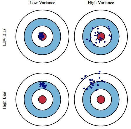
• Here, suppose:
  • The red bulls-eye represents your true weight and height 🧍.
  • The dark blue darts represent predictions of your weight and height using different models that were fit using different samples drawn from the same population.

• We'd like our models to be in the top left, but in practice that's hard to achieve!

Risk vs. empirical risk

• Since Lecture 11, we've minimized empirical risk to find optimal model parameters $\vec{w}^*$:

$$\vec{w}^* = \underset{\vec{w}}{\text{argmin}} \frac{1}{n} \sum_{i = 1}^n \left( y_i - H(\vec x_i) \right)^2$$

• Key idea: A model that works well on past data should work well on future data, if future data looks like past data.

• What we really want is for the:

  • expected loss for a new data point $(\vec x_{\text{new}}, y_{\text{new}})$,
  • drawn from the same population as the training set, to be small.

  That is, we want to minimize risk: $$\text{risk} = \mathbb{E}[y_{\text{new}} - H(\vec x_{\text{new}})]^2$$

• In general, we don't know the entire population distribution of $x$s and $y$s, so we can't compute risk exactly.
  That's why we compute empirical risk!

$$\mathbb{E}[y_{\text{new}} - H(\vec x_{\text{new}})]^2 \approx \frac{1}{n} \sum_{i = 1}^n \left( y_i - H(\vec x_i) \right)^2 = R(H)$$

The bias-variance decomposition

• Risk can be decomposed as follows:
  Remember, this expectation $\mathbb{E}$ is over the entire population of $x$s and $y$s. In real life, we don't know what this population distribution is, so we can't put actual numbers to this.

$$\mathbb{E}[y_{\text{new}} - H(\vec x_{\text{new}})]^2 = \text{model bias}^2 + \text{model variance} + \text{observation error}$$

• We won't cover the proof of the decomposition here – read this for more – but note that in Homework 6, Question 3, you proved a related formula for $R_\text{sq}(h)$:

$$R_\text{sq}(h) = \frac{1}{n} \sum_{i = 1}^n (y_i - h)^2 = \underbrace{\frac{1}{n} \sum_{i = 1}^n (y_i - \bar{y})^2}_{\text{variance of } y} + (\bar{y} - h)^2$$

• Key takeaway: If we care about minimizing (empirical) risk, we can equivalently try to minimize both model bias and model variance.

• As model variance increases, model bias tends to decrease, and vice versa.
  That is, there is a tradeoff between bias and variance:

Hyperparameters and train-test splits 🎛️

---

Example: Polynomial regression

• We recently looked at an example of polynomial regression.

fig = util.train_and_plot(train_sample=sample_1, test_sample=sample_2, degs=[1, 3, 25], data_name='Sample 2')
fig.update_layout(title='Trained on Sample 1, Performance on Sample 2')

• When building these models:
  • We got to choose the degree of the polynomials – we chose 1, 3, and 25.
  • We didn't get to choose the exact formulas for the three polynomials – their formulas were learned from data.
    No matter what the data looked like, the left-most model had to look like a line, because we chose its degree in advance.

Hyperparameters

• A parameter defines the relationship between variables in a model. We learn parameters from data.

  • For instance, suppose we fit a degree 3 polynomial to data, and end up with:

  $$H^*(x_i) = 1 - 2x_i + 13x_i^2 - 4x_i^3$$

  • 1, -2, 13, and -4 are parameters.

• A hyperparameter is a parameter that we choose before our model is fit to the data.
  • Think of hyperparameters as knobs 🎛 – we get to pick and tune them!
  • Polynomial degree was a hyperparameter in the previous example, and we tried three different values: 1, 3, and 25.

• Question: How do we choose the "right" hyperparameter(s)?
  Degree 3 was a better choice than degree 25, for example – but how do we systematically choose?

Train-test splits 🚆

• Suppose we're choosing between many different models.
  Here, by "model" we really mean "hyperparameter value", e.g. one "model" is a degree 3 polynomial, while another is a degree 4 polynomial.

• We won't know whether a model has overfit to our sample unless we get to see how well it performs on a new sample from the same population.

• 💡Idea: Split our dataset into a training set and test set.

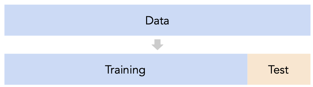
• For each model we're considering (e.g. each polynomial degree):
  • Use only the training set to fit that model (i.e. find $\vec{w}^*$).
  • Use the test set to evaluate that model's error (e.g. compute its MSE).

• Pick the model with the lowest test error.

• Why? The test set is like a new sample of data from the same population as the training data!

Train-test split

• sklearn.model_selection.train_test_split implements a train-test split for us! 🙏🏼

• If X is an array/DataFrame of features and y is an array/Series of responses,

  X_train, X_test, y_train, y_test = train_test_split(X, y, test_size=0.25)
  

  randomly splits the features and responses into training and test sets, such that the test set contains 0.25 of the full dataset.

from sklearn.model_selection import train_test_split

# Read the documentation!
train_test_split?

• Let's perform a train/test split on sample_1, since we'll need it to find the optimal polynomial degree.

sample_1

	x	y
0	-2.00	-6.00
1	-1.95	-7.33
2	-1.90	-9.18
...	...	...
97	2.90	25.75
98	2.95	22.40
99	3.00	32.47

100 rows × 2 columns

X = sample_1[['x']] # DataFrame. 
y = sample_1['y'] # Series. 
# We don't have to choose 0.25.
# We also don't have to set a random_state;
# we've done this so that we get the same results in lecture every time.
X_train, X_test, y_train, y_test = train_test_split(X, y, test_size=0.2, random_state=23) 

• Before proceeding, let's check the sizes of X_train and X_test.

print('Rows in X_train:', X_train.shape[0])
display(X_train.head())
print('Rows in X_test:', X_test.shape[0])
display(X_test.head())

Rows in X_train: 80

	x
85	2.29
28	-0.59
8	-1.60
11	-1.44
63	1.18

Rows in X_test: 20

	x
26	-0.69
80	2.04
82	2.14
68	1.43
77	1.89

Remember: Train only using the training data!

• Now that we've performed a train/test split of Sample 1, we'll create models with degree 1 through 25 polynomial features and compute their train and test errors.

from sklearn.pipeline import Pipeline, make_pipeline
from sklearn.linear_model import LinearRegression
from sklearn.metrics import mean_squared_error
train_errs = []
test_errs = []
for d in range(1, 26):
    pl = make_pipeline(PolynomialFeatures(d), LinearRegression())
    pl.fit(X_train, y_train)
    train_errs.append(mean_squared_error(y_train, pl.predict(X_train)))
    test_errs.append(mean_squared_error(y_test, pl.predict(X_test)))
errs = pd.DataFrame({'Train Error': train_errs, 'Test Error': test_errs})
errs

	Train Error	Test Error
0	20.86	20.79
1	13.08	14.31
2	7.01	12.10
...	...	...
22	5.27	14.26
23	5.10	14.64
24	65.22	63.25

25 rows × 2 columns

• Notice that we only call pl.fit on the training data!

Polynomial degree vs. train/test error

• Let's look at the plots of training error vs. degree and test error vs. degree.

fig = px.line(errs.iloc[:-1])
fig.update_layout(showlegend=True, xaxis_title='Polynomial Degree', yaxis_title='Mean Squared Error')

• Training error appears to decrease as polynomial degree increases.

• Test error appears to decrease until a "valley", and then increases again.

• Here, we'd choose a degree of 3, since that degree has the lowest test error.

Training error vs. test error

• The pattern we saw in the previous example is true more generally.

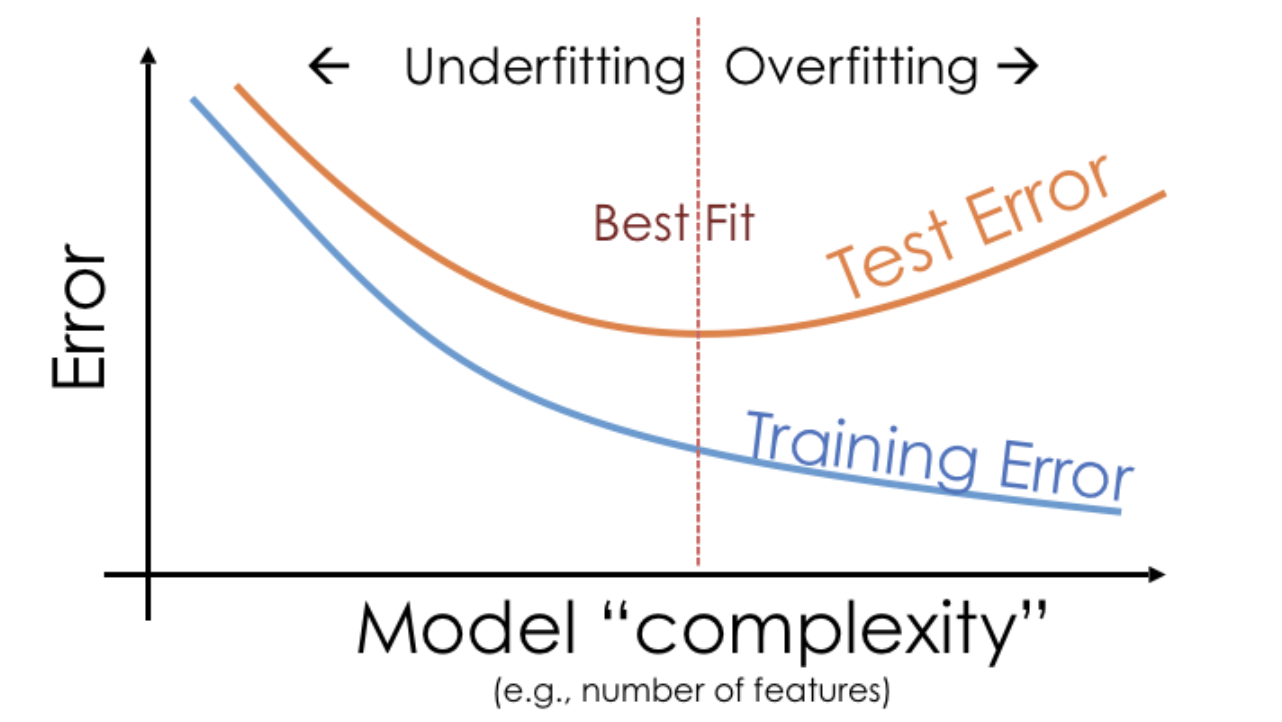
• We pick the hyperparameter(s) at the "valley" of test error.

• Note that training error tends to underestimate test error, but it doesn't have to – i.e., it is possible for test error to be lower than training error (say, if the test set is "easier" to predict than the training set).

• The results – and the bias-variance tradeoff more generally – hold true for "classic" machine learning models, like the ones we're studying here.
  But in deep neural networks, this pattern is often violated; extremely complex models can have low test error as well.
  This phenomenon is known as "double descent"; learn more here.

Conducting train-test splits

• Recall, training data is used to fit our model, and test data is used to evaluate our model.

• Question: How should we split?
  • sklearn's train_test_split splits randomly, which usually works well.
  • However, if there is some element of time in the training data (say, when predicting the future price of a stock), a better split is "past" and "future".

• Question: How large should the split be, e.g. 90%-10% vs. 75%-25%?
  • There's a tradeoff – a larger training set should lead to a "better" model, while a larger test set should lead to a better estimate of our model's ability to generalize.
  • There's no "right" choice, but we usually choose between 10% to 25% for the test set.

But wait...

• With our current strategy, we are choosing the hyperparameter that creates the model that performs best on the test set.

• As such, we are overfitting to the test set – the best hyperparameter for the test set might not be the best hyperparameter for a totally unseen dataset!

• It seems like we need another split.

Cross-validation

---

Idea: A single validation set

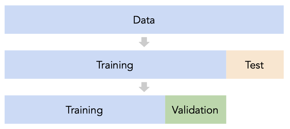
1. Split the data into three sets: training, validation, and test.

2. For each hyperparameter choice, train the model only on the training set, and evaluate the model's performance on the validation set.

3. Find the hyperparameter with the best validation performance.

4. Retrain the final model on the training and validation sets, and report its performance on the test set.

• Issue: This strategy is too dependent on the validation set, which may be small and/or not a representative sample of the data. We're not going to do this. ❌

A better idea: $k$-fold cross-validation

• Instead of relying on a single validation set, we can create $k$ validation sets, where $k$ is some positive integer (5 in the example below).

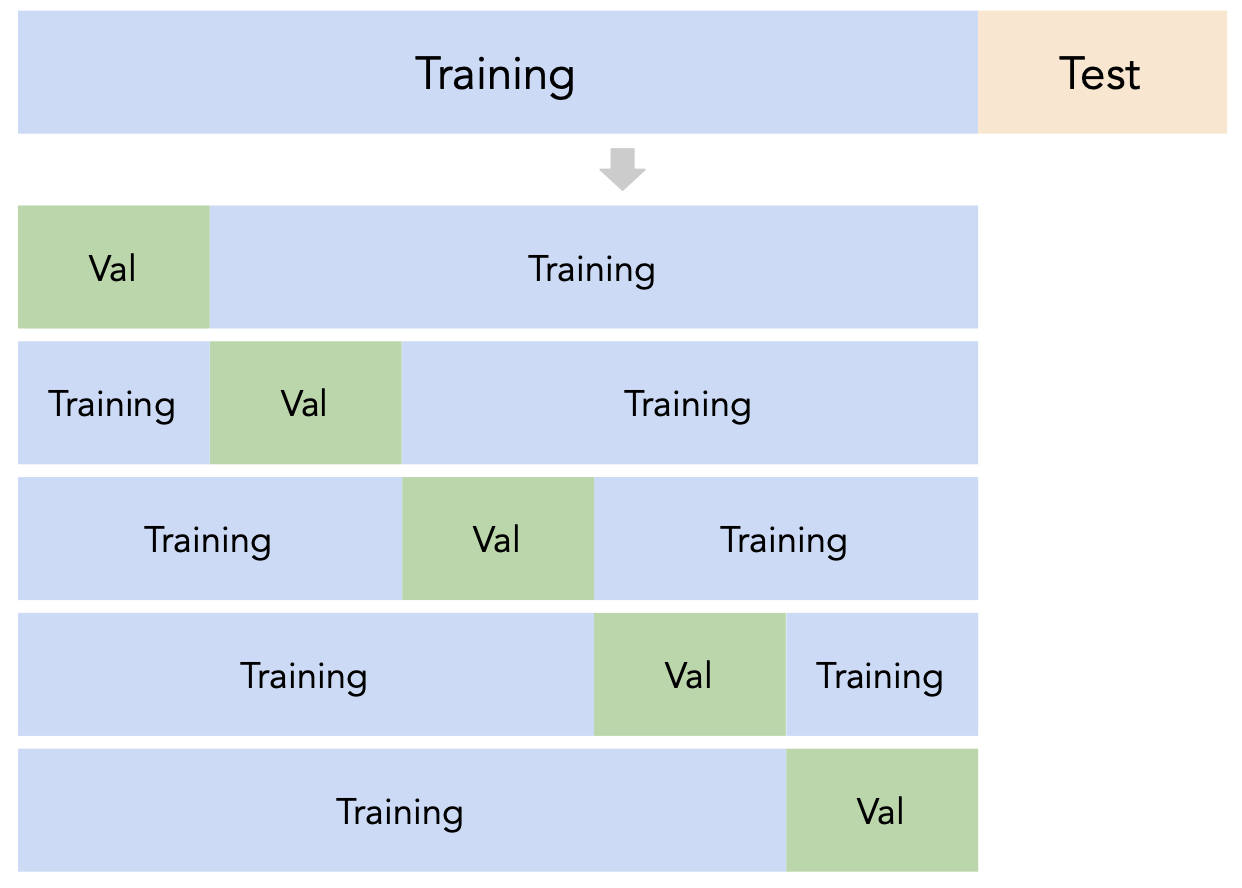
• Since each data point is used for training $k-1$ times and validation once, the (averaged) validation performance should be a good metric of a model's ability to generalize to unseen data.

• $k$-fold cross-validation (or simply "cross-validation") is the technique we will use for finding hyperparameters, or more generally, for choosing between different possible models. It's what you should use in your Final Project! ✅

Illustrating $k$-fold cross-validation

• To illustrate $k$-fold cross-validation, let's use the following example dataset with $n = 12$ rows.
  Suppose this dataset represents our training set, i.e. suppose we already performed a train-test split.

training_data = pd.DataFrame().assign(x=range(0, 120, 10),
                                      y=[9, 1, 58, 3, 6, 4, -2, 8, 1, 10, 1.1, -45])        
display_df(training_data, rows=12)

	x	y
0	0	9.0
1	10	1.0
2	20	58.0
3	30	3.0
4	40	6.0
5	50	4.0
6	60	-2.0
7	70	8.0
8	80	1.0
9	90	10.0
10	100	1.1
11	110	-45.0

• Suppose we choose $k = 4$. Then, each fold has $\frac{12}{4} = 3$ rows.

show_cv_slides()

$k$-fold cross-validation, in general

• First, shuffle the entire training set randomly and split it into $k$ disjoint folds, or "slices". Then:

• For each hyperparameter:
  • For each slice:
    • Let the slice be the "validation set", $V$.
    • Let the rest of the data be the "training set", $T$.
    • Train a model using the selected hyperparameter on the training set $T$.
    • Evaluate the model on the validation set $V$.
  • Compute the average validation error (e.g. MSE) for the particular hyperparameter.

• Choose the hyperparameter with the lowest average validation error.

GridSearchCV

• Let's use $k$-fold cross-validation to choose a polynomial degree that best generalizes to unseen data.
  As before, we'll choose our polynomial degree from the list [1, 2, ..., 25].

• GridSearchCV takes in:

  • an un-fit instance of an estimator, and
  • a dictionary of hyperparameter values to try,

  and performs $k$-fold cross-validation to find the combination of hyperparameters with the best average validation performance.

from sklearn.model_selection import GridSearchCV
GridSearchCV?

• Why do you think it's called "grid search"?

Grid searching for the best polynomial degree

• Here, we want to try values of degree from 1 through 25, so we'll need to specify these values in a dictionary.

# The key names in this dictionary are chosen very carefully.
# They need to be of the format pipelinestep__hyperparametername,
# where pipelinestep is a lowercase version of the step in the pipeline
# that we want to tune, and 
# hyperparameter name is the formal name of the hyperparameter (see the documentation).
hyperparams = {
    'polynomialfeatures__degree': range(1, 26)
}

• The scoring metric we need to provide is 'neg_mean_squared_error'.
  The scoring argument is used to specify that we want to compute the MSE; by default, it computes the $R^2$. It's called "neg" MSE because, by default, sklearn likes to "maximize" scores, and maximizing -MSE is the same as minimizing MSE.

searcher = GridSearchCV(
    make_pipeline(PolynomialFeatures(), LinearRegression()),
    param_grid=hyperparams,
    cv=5, # k = 5.
    scoring='neg_mean_squared_error'
)
searcher

GridSearchCV(cv=5,
             estimator=Pipeline(steps=[('polynomialfeatures',
                                        PolynomialFeatures()),
                                       ('linearregression',
                                        LinearRegression())]),
             param_grid={'polynomialfeatures__degree': range(1, 26)},
             scoring='neg_mean_squared_error')

In a Jupyter environment, please rerun this cell to show the HTML representation or trust the notebook.
On GitHub, the HTML representation is unable to render, please try loading this page with nbviewer.org.

• Like any other estimator, GridSearchCV instances need to be fit.
  Again, notice that we're only fitting it with our training data.

searcher.fit(X_train, y_train)

GridSearchCV(cv=5,
             estimator=Pipeline(steps=[('polynomialfeatures',
                                        PolynomialFeatures()),
                                       ('linearregression',
                                        LinearRegression())]),
             param_grid={'polynomialfeatures__degree': range(1, 26)},
             scoring='neg_mean_squared_error')

In a Jupyter environment, please rerun this cell to show the HTML representation or trust the notebook.
On GitHub, the HTML representation is unable to render, please try loading this page with nbviewer.org.

• Once fit, searcher can tell us what it found!

searcher.best_params_

{'polynomialfeatures__degree': 3}

• searcher is now a fit regression model. There's no need to refit it on the entire training set; it was already fit on the entire training set automatically.

searcher.predict([[4], 
                  [-1], 
                  [0]])

array([64.62, -1.22,  0.32])

Interpreting the results of $k$-fold cross-validation

• Let's peek under the hood.

errs_df = util.format_results(searcher)
errs_df

	Degree 1	Degree 2	Degree 3	Degree 4	...	Degree 22	Degree 23	Degree 24	Degree 25
Fold 1	22.54	15.35	6.93	7.15	...	46.38	64.23	35.50	102.93
Fold 2	30.24	18.46	8.42	12.15	...	560.61	630.02	1596.78	4589.27
Fold 3	15.93	11.42	4.47	4.62	...	304.46	198.77	643.80	31566.25
Fold 4	26.99	17.79	12.99	13.02	...	15.29	15.76	15.24	28.90
Fold 5	11.24	4.58	4.66	5.16	...	8.39	7.95	8.18	64.57

5 rows × 25 columns

• Note that for each choice of degree (our hyperparameter), we have five MSEs, one for each "fold" of the data. This means that in total, $5 \cdot 25 = 125$ models were trained!

errs_df

	Degree 1	Degree 2	Degree 3	Degree 4	...	Degree 22	Degree 23	Degree 24	Degree 25
Fold 1	22.54	15.35	6.93	7.15	...	46.38	64.23	35.50	102.93
Fold 2	30.24	18.46	8.42	12.15	...	560.61	630.02	1596.78	4589.27
Fold 3	15.93	11.42	4.47	4.62	...	304.46	198.77	643.80	31566.25
Fold 4	26.99	17.79	12.99	13.02	...	15.29	15.76	15.24	28.90
Fold 5	11.24	4.58	4.66	5.16	...	8.39	7.95	8.18	64.57

5 rows × 25 columns

• Remember, our goal is to choose the degree with the lowest average validation error.

errs_df.mean(axis=0)

Degree 1       21.39
Degree 2       13.52
Degree 3        7.49
              ...   
Degree 23     183.34
Degree 24     459.90
Degree 25    7270.38
Length: 25, dtype: float64

fig = errs_df.mean(axis=0).iloc[:18].plot(kind='line', title='Average Validation Error')
fig.update_layout(xaxis_title='Degree', yaxis_title='Average Validation MSE', showlegend=False)

# Chosen automatically by sklearn.
errs_df.mean(axis=0).idxmin()

'Degree 3'

• Note that if we didn't perform $k$-fold cross-validation, but instead just used a single validation set, we may have ended up with a different result:

errs_df.idxmin(axis=1)

Fold 1     Degree 6
Fold 2     Degree 3
Fold 3    Degree 12
Fold 4    Degree 10
Fold 5     Degree 2
dtype: object

Question 🤔 (Answer at practicaldsc.org/q)

• Suppose you have a training dataset with 1000 rows.
• You want to decide between 20 hyperparameters for a particular model.
• To do so, you perform 10-fold cross-validation.
• How many times is the first row in the training dataset (X.iloc[0]) used for training a model?

Another example: Commute times

• We can also use $k$-fold cross-validation to determine which subset of features to use in a linear model that predicts commute times!

df = pd.read_csv('data/commute-times.csv')
df['day_of_month'] = pd.to_datetime(df['date']).dt.day
df['month'] = pd.to_datetime(df['date']).dt.month_name()
df.head()

	date	day	home_departure_time	home_departure_mileage	...	work_departure_time_hr	mileage_to_home	day_of_month	month
0	5/15/2023	Mon	2023-05-15 10:49:00	15873.0	...	17.17	53.0	15	May
1	5/16/2023	Tue	2023-05-16 07:45:00	15979.0	...	NaN	NaN	16	May
2	5/22/2023	Mon	2023-05-22 08:27:00	50407.0	...	15.90	54.0	22	May
3	5/23/2023	Tue	2023-05-23 07:08:00	50535.0	...	NaN	NaN	23	May
4	5/30/2023	Tue	2023-05-30 09:09:00	50664.0	...	17.12	54.0	30	May

5 rows × 20 columns

• Let's make several candidate pipelines. But first, as always, a train-test split.

# Here, we're letting X_train and X_test keep all of the columns in the DataFrame
# OTHER than 'minutes'.
X_train, X_test, y_train, y_test = train_test_split(df.drop('minutes', axis=1), df['minutes'], random_state=23)

Creating many pipelines

from sklearn.compose import make_column_transformer, make_column_selector
from sklearn.preprocessing import FunctionTransformer, OneHotEncoder

selecter = FunctionTransformer(lambda x: x) # Shortcut to say "keep just these columns."
week_converter = FunctionTransformer(lambda s: 'Week ' + ((s - 1) // 7 + 1).astype(str))
day_of_month_transformer = make_pipeline(week_converter, OneHotEncoder(drop='first')) # From last class.
pipes = {
    'departure_hour only': make_pipeline(
        make_column_transformer((selecter, ['departure_hour'])),
        LinearRegression()
    ),
    'departure_hour + day_of_month': make_pipeline(
        make_column_transformer((selecter, ['departure_hour', 'day_of_month'])),
        LinearRegression()
    ),
    'departure_hour + day OHE': make_pipeline(
        make_column_transformer(
            (selecter, ['departure_hour']),
            (OneHotEncoder(drop='first', handle_unknown='ignore'), ['day'])
        ),
        LinearRegression()
    ),
    'departure_hour + day OHE + month OHE': make_pipeline(
        make_column_transformer(
            (selecter, ['departure_hour']),
            (OneHotEncoder(drop='first', handle_unknown='ignore'), ['day', 'month'])
        ),
        LinearRegression()
    ),
    'departure_hour with poly features + day OHE + month OHE + week': make_pipeline(
        make_column_transformer(
        (PolynomialFeatures(3), ['departure_hour']),
        (OneHotEncoder(drop='first', handle_unknown='ignore'), ['day', 'month']),
        (day_of_month_transformer, ['day_of_month']),
    ),
    LinearRegression())
}

• Here, we will have to call GridSearchCV multiple times.
  Here, we're choosing between many different pipelines, not between hyperparameters for a particular pipeline.

results = pd.DataFrame(columns=['Average Training MSE', 'Average Validation MSE'])
for pipe in pipes:
    fitted = GridSearchCV(
        pipes[pipe],
        param_grid={}, # No hyperparameters, but we could have them.
        scoring='neg_mean_squared_error',
        cv=10, # Change this and see what happens!
        return_train_score=True # So that we can compute training MSEs, too.
    )
    fitted.fit(X_train, y_train)
    results.loc[pipe] = [-fitted.cv_results_['mean_train_score'][0], -fitted.cv_results_['mean_test_score'][0]]
commute_models_summarized = (
    results
    .sort_values('Average Training MSE')
    .plot(kind='barh', barmode='group', width=1000)
    .update_layout(xaxis_title='Mean Squared Error', yaxis_title='Model')
)
commute_models_summarized

• What's the "right" combination of features to choose?

Summary

• We care about how well our models generalize to unseen data.
  
  • The more complex a model is, the more it will overfit to the noise in the training data, and have high model variance.
  • The less complex a model is, the more it will underfit the training data, and have high bias.

• To navigate this bias-variance tradeoff, we choose model complexity by choosing the model with the lowest error on unseen data.

• To do so, use cross-validation:
  1. Split the data into two sets: training and test.
  2. Use only the training data when designing, training, and tuning the model.
     • Use $k$-fold cross-validation to choose hyperparameters and estimate the model's ability to generalize.
     • Do not ❌ look at the test data in this step!
  3. Commit to your final model and train it using the entire training set.
  4. Test the data using the test data. If the performance (e.g. MSE) is not acceptable, return to step 2.
  5. Finally, train on all available data and ship the model to production! 🛳

• 🚨 This is the process you should always use! 🚨

Question 🤔 (Answer at practicaldsc.org/q)

What questions do you have?