from lec_utils import *
Lecture 16
Feature Engineering
EECS 398: Practical Data Science, Spring 2025
practicaldsc.org • github.com/practicaldsc/sp25 • 📣 See latest announcements here on Ed
Agenda 📆
- Recap: Multiple linear regression.
- Feature engineering.
- Numerical-to-numerical transformations 🧬.
- The modeling recipe, revisited.
StandardScalerand standardized regression coefficients.
Question 🤔 (Answer at practicaldsc.org/q)
Remember that you can always ask questions anonymously at the link above!
Recap: Multiple linear regression
The general problem
- We have $n$ data points, $\left({ \vec x_1}, {y_1}\right), \left({ \vec x_2}, {y_2}\right), \ldots, \left({ \vec x_n}, {y_n}\right)$,
where each $ \vec x_i$ is a feature vector of $d$ features: $${\vec{x_i}} = \begin{bmatrix} {x^{(1)}_i} \\ {x^{(2)}_i} \\ \vdots \\ {x^{(d)}_i} \end{bmatrix}$$
- We want to find a good linear hypothesis function:
- Specifically, we want to find the optimal parameters, $w_0^*$, $w_1^*$, ..., $w_d^*$ that minimize mean squared error:
The general solution
- Define the design matrix $ X \in \mathbb{R}^{n \times (d + 1)}$ and observation vector $\vec y \in \mathbb{R}^n$:
- Then, solve the normal equations to find the optimal parameter vector, $\vec{w}^*$:
- The $\vec w^*$ that satisfies the equations above minimizes mean squared error, $R_\text{sq}(\vec w)$, so use this $\vec w^*$ to make predictions.
- Once $\vec w^*$ is found:
- $X \vec w^*$ is a hypothesis vector of predicted $y$-values for the entire dataset.
- $$H^*(\vec x_i) = w_0^* + w_1^* x_i^{(1)} + w_2^* x_i^{(2)} + ... + w_d^* x_i^{(d)} = \vec w^* \text{Aug}(\vec x_i)$$returns the predicted $y$-value for just the input $\vec x_i$.
- If $X^TX$ is invertible, then:
sklearncan compute $\vec w^*$ automatically, as we will see again shortly.
Feature engineering ⚙️
The goal of feature engineering
- Feature engineering is the act of finding transformations that transform data into effective quantitative variables.
Put simply: feature engineering is creating new features using existing features.
- Example: One hot encoding.
- Example: Numerical-to-numerical transformations.
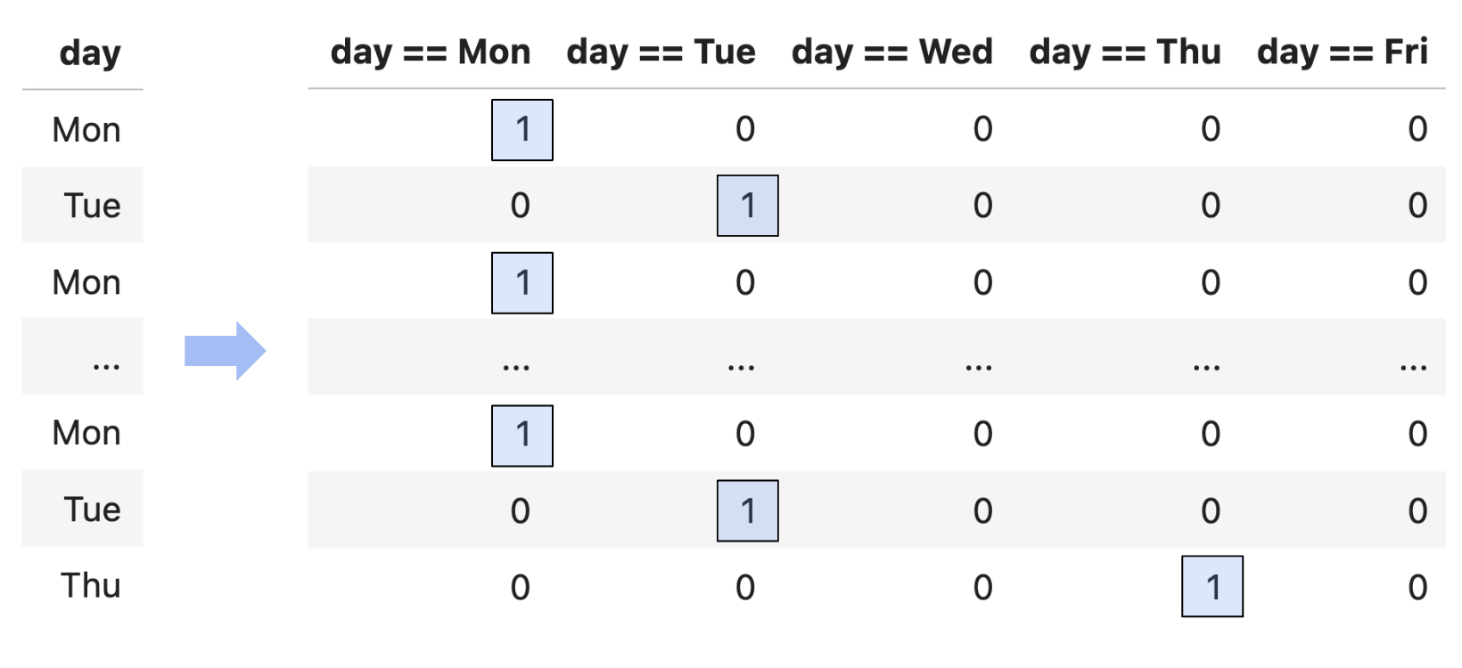
One hot encoding
- One hot encoding is a transformation that turns a categorical feature into several binary features.
- Suppose a column has $N$ unique values, $A_1$, $A_2$, ..., $A_N$. For each unique value $A_i$, we define the following feature function:
- Note that 1 means "yes" and 0 means "no".
- One hot encoding is also called "dummy encoding", and $\phi_i(x)$ may also be referred to as an "indicator variable".
Run the cells below to set up the next slide.
df = pd.read_csv('data/commute-times.csv')
df['day_of_month'] = pd.to_datetime(df['date']).dt.day
df.head()
| date | day | home_departure_time | home_departure_mileage | ... | minutes_to_home | work_departure_time_hr | mileage_to_home | day_of_month | |
|---|---|---|---|---|---|---|---|---|---|
| 0 | 5/15/2023 | Mon | 2023-05-15 10:49:00 | 15873.0 | ... | 72.0 | 17.17 | 53.0 | 15 |
| 1 | 5/16/2023 | Tue | 2023-05-16 07:45:00 | 15979.0 | ... | NaN | NaN | NaN | 16 |
| 2 | 5/22/2023 | Mon | 2023-05-22 08:27:00 | 50407.0 | ... | 82.0 | 15.90 | 54.0 | 22 |
| 3 | 5/23/2023 | Tue | 2023-05-23 07:08:00 | 50535.0 | ... | NaN | NaN | NaN | 23 |
| 4 | 5/30/2023 | Tue | 2023-05-30 09:09:00 | 50664.0 | ... | 76.0 | 17.12 | 54.0 | 30 |
5 rows × 19 columns
Example: One hot encoding 'day'
- For each unique value of
'day'in our dataset, we must create a column for just that'day'.
df.head()
| date | day | home_departure_time | home_departure_mileage | ... | minutes_to_home | work_departure_time_hr | mileage_to_home | day_of_month | |
|---|---|---|---|---|---|---|---|---|---|
| 0 | 5/15/2023 | Mon | 2023-05-15 10:49:00 | 15873.0 | ... | 72.0 | 17.17 | 53.0 | 15 |
| 1 | 5/16/2023 | Tue | 2023-05-16 07:45:00 | 15979.0 | ... | NaN | NaN | NaN | 16 |
| 2 | 5/22/2023 | Mon | 2023-05-22 08:27:00 | 50407.0 | ... | 82.0 | 15.90 | 54.0 | 22 |
| 3 | 5/23/2023 | Tue | 2023-05-23 07:08:00 | 50535.0 | ... | NaN | NaN | NaN | 23 |
| 4 | 5/30/2023 | Tue | 2023-05-30 09:09:00 | 50664.0 | ... | 76.0 | 17.12 | 54.0 | 30 |
5 rows × 19 columns
df['day'].value_counts()
day
Tue    25
Mon    20
Thu    15
Wed     3
Fri     2
Name: count, dtype: int64
(df['day'] == 'Tue').astype(int)
0     0
1     1
2     0
     ..
62    0
63    1
64    0
Name: day, Length: 65, dtype: int64
for val in df['day'].unique():
    df[f'day == {val}'] = (df['day'] == val).astype(int)
df.loc[:, df.columns.str.contains('day')]
| day | day_of_month | day == Mon | day == Tue | day == Wed | day == Thu | day == Fri | |
|---|---|---|---|---|---|---|---|
| 0 | Mon | 15 | 1 | 0 | 0 | 0 | 0 |
| 1 | Tue | 16 | 0 | 1 | 0 | 0 | 0 |
| 2 | Mon | 22 | 1 | 0 | 0 | 0 | 0 |
| ... | ... | ... | ... | ... | ... | ... | ... |
| 62 | Mon | 4 | 1 | 0 | 0 | 0 | 0 |
| 63 | Tue | 5 | 0 | 1 | 0 | 0 | 0 |
| 64 | Thu | 7 | 0 | 0 | 0 | 1 | 0 |
65 rows × 7 columns
Using 'day' as a feature, along with 'departure_hour' and 'day_of_month'
- Now that we've converted
'day'to a numerical variable, we can use it as input in a regression model. Here's the model we'll try to fit:
- Subtlety: Since there are only 5 values of
'day', we don't need to include $\text{day}_i \text{ == Fri}$ as a feature. We know it's Friday if $\text{day}_i \text{ == Mon}$, $\text{day}_i \text{ == Tue}$, ... are all 0.
More on this next class!
X_for_ohe = df[['departure_hour',
                'day_of_month',
                'day == Mon',
                'day == Tue',
                'day == Wed',
                'day == Thu']]
X_for_ohe
| departure_hour | day_of_month | day == Mon | day == Tue | day == Wed | day == Thu | |
|---|---|---|---|---|---|---|
| 0 | 10.82 | 15 | 1 | 0 | 0 | 0 |
| 1 | 7.75 | 16 | 0 | 1 | 0 | 0 |
| 2 | 8.45 | 22 | 1 | 0 | 0 | 0 |
| ... | ... | ... | ... | ... | ... | ... |
| 62 | 7.58 | 4 | 1 | 0 | 0 | 0 |
| 63 | 7.45 | 5 | 0 | 1 | 0 | 0 |
| 64 | 7.60 | 7 | 0 | 0 | 0 | 1 |
65 rows × 6 columns
from sklearn.linear_model import LinearRegression
model_with_ohe = LinearRegression()
model_with_ohe.fit(X=X_for_ohe, y=df['minutes'])
LinearRegression()In a Jupyter environment, please rerun this cell to show the HTML representation or trust the notebook.
On GitHub, the HTML representation is unable to render, please try loading this page with nbviewer.org.
LinearRegression()
- The following cell gives us our $w^*$s:
model_with_ohe.intercept_, model_with_ohe.coef_
(134.0430659240799, array([-8.42, -0.03, 5.09, 16.38, 5.12, 11.5 ]))
- Thus, our trained linear model to predict commute time given
'departure_hour','day_of_month', and'day'(Mon, Tue, Wed, or Thu) is:
Visualizing our latest model
- Our trained linear model to predict commute time given
'departure_hour','day_of_month', and'day'(Mon, Tue, Wed, or Thu) is:
- Since we have 6 features here, we'd need 7 dimensions to graph our model.
- But, as we see in Homework 7, Question 5, our model is really a collection of five parallel planes in 3D, all with slightly different $z$-intercepts!
- If we want to visualize in 2D, we need to pick a single feature to place on the $x$-axis.
fig = go.Figure()
fig.add_trace(go.Scatter(x=df['departure_hour'], y=df['minutes'],
                         mode='markers', name='Original Data'))
fig.add_trace(go.Scatter(x=df['departure_hour'], y=model_with_ohe.predict(X_for_ohe),
                         mode='markers', name='Predicted Commute Times using Departure Hour, <br>Day of Month, and Day of Week'))
fig.update_layout(showlegend=True, title='Commute Time vs. Departure Hour',
                  xaxis_title='Departure Hour', yaxis_title='Minutes', width=1000)
- Despite being a linear model, why doesn't this model look like a straight line?
Run the cells below to set up the next slide.
from sklearn.metrics import mean_squared_error
# Multiple linear regression model.
model_multiple = LinearRegression()
model_multiple.fit(X=df[['departure_hour', 'day_of_month']], y=df['minutes'])
mse_dict = {}
mse_dict['departure_hour + day_of_month'] = mean_squared_error(df['minutes'], model_multiple.predict(df[['departure_hour', 'day_of_month']]))
# Simple linear model.
model_simple = LinearRegression()
model_simple.fit(X=df[['departure_hour']], y=df['minutes'])
mse_dict['departure_hour'] = mean_squared_error(df['minutes'], model_simple.predict(df[['departure_hour']]))
# Constant model.
model_constant = df['minutes'].mean()
mse_dict['constant'] = mean_squared_error(df['minutes'], np.ones(df.shape[0]) * model_constant)
Comparing our latest model to earlier models
- Let's see how the inclusion of the day of the week impacts the quality of our predictions.
mse_dict['departure_hour + day_of_month + ohe day'] = mean_squared_error(
    df['minutes'],
    model_with_ohe.predict(X_for_ohe)
)
pd.Series(mse_dict).plot(kind='barh', title='Mean Squared Error')
- Adding the day of the week decreased our MSE significantly!
Reflection
df.head()
| date | day | home_departure_time | home_departure_mileage | ... | day == Tue | day == Wed | day == Thu | day == Fri | |
|---|---|---|---|---|---|---|---|---|---|
| 0 | 5/15/2023 | Mon | 2023-05-15 10:49:00 | 15873.0 | ... | 0 | 0 | 0 | 0 |
| 1 | 5/16/2023 | Tue | 2023-05-16 07:45:00 | 15979.0 | ... | 1 | 0 | 0 | 0 |
| 2 | 5/22/2023 | Mon | 2023-05-22 08:27:00 | 50407.0 | ... | 0 | 0 | 0 | 0 |
| 3 | 5/23/2023 | Tue | 2023-05-23 07:08:00 | 50535.0 | ... | 1 | 0 | 0 | 0 |
| 4 | 5/30/2023 | Tue | 2023-05-30 09:09:00 | 50664.0 | ... | 1 | 0 | 0 | 0 |
5 rows × 24 columns
- We've one hot encoded
'day', but it required afor-loop.
- Is there a way we could have encoded it without a
for-loop?
- Yes, using
sklearn.preprocessing'sOneHotEncoder. More on this soon!
Question 🤔 (Answer at practicaldsc.org/q)
Remember that you can always ask questions anonymously at the link above!
Numerical-to-numerical transformations 🧬
Example: Horsepower 🚗
- The following dataset, built into the
seabornplotting library, contains various information about (older) cars.
import seaborn as sns
mpg = sns.load_dataset('mpg').dropna()
mpg.head()
| mpg | cylinders | displacement | horsepower | ... | acceleration | model_year | origin | name | |
|---|---|---|---|---|---|---|---|---|---|
| 0 | 18.0 | 8 | 307.0 | 130.0 | ... | 12.0 | 70 | usa | chevrolet chevelle malibu |
| 1 | 15.0 | 8 | 350.0 | 165.0 | ... | 11.5 | 70 | usa | buick skylark 320 |
| 2 | 18.0 | 8 | 318.0 | 150.0 | ... | 11.0 | 70 | usa | plymouth satellite |
| 3 | 16.0 | 8 | 304.0 | 150.0 | ... | 12.0 | 70 | usa | amc rebel sst |
| 4 | 17.0 | 8 | 302.0 | 140.0 | ... | 10.5 | 70 | usa | ford torino |
5 rows × 9 columns
- We really do mean old:
mpg['model_year'].value_counts()
model_year
73    40
78    36
76    34
      ..
71    27
80    27
74    26
Name: count, Length: 13, dtype: int64
- Let's investigate the relationship between
'horsepower'and'mpg'.
The relationship between 'horsepower' and 'mpg'
px.scatter(mpg, x='horsepower', y='mpg')
- It appears that there is a negative association between
'horsepower'and'mpg', though it's not quite linear.
- Let's try and fit a simple linear model that uses
'horsepower'to predict'mpg'and see what happens.
Predicting 'mpg' using 'horsepower'
car_model = LinearRegression()
car_model.fit(mpg[['horsepower']], mpg['mpg'])
LinearRegression()In a Jupyter environment, please rerun this cell to show the HTML representation or trust the notebook.
On GitHub, the HTML representation is unable to render, please try loading this page with nbviewer.org.
LinearRegression()
- What do our predictions look like?
hp_points = pd.DataFrame({'horsepower': [25, 225]})
fig = px.scatter(mpg, x='horsepower', y='mpg')
fig.add_trace(go.Scatter(
    x=hp_points['horsepower'],
    y=car_model.predict(hp_points),
    mode='lines',
    name='Predicted MPG using Horsepower'
))
- Our regression line doesn't capture the curvature in the relationship between
'horsepower'and'mpg'.
# As a baseline:
mean_squared_error(mpg['mpg'], car_model.predict(mpg[['horsepower']]))
23.943662938603108
Linear in the parameters
Using linear regression, we can fit hypothesis functions like: $$ H(x_i) = w_0 + w_1x_i+w_2x_i^2 \qquad \qquad H(\vec x_i) = w_1e^{-x_i^{{(1)}^2}} + w_2 \cos(x_i^{(2)}+\pi) +w_3 \frac{\log 2x_i^{(3)}}{x_i^{(2)}} $$
This includes all polynomials, for example. These are all linear combinations of (just) features.
- For any of the above examples, we could express our model as $\vec w \cdot \text{Aug} (\vec x_i)$, for some carefully chosen feature vector $\vec x_i$,
and that's all thatLinearRegressioninsklearnneeds.
What we put in theXargument tomodel.fitis up to us!
- Using linear regression, we can't fit hypothesis functions like:
$$
H(x_i) = w_0 + e^{w_1 x_i}
\qquad \qquad
H(\vec x_i) = w_0 + \sin (w_1 x_i^{(1)} + w_2 x_i^{(2)})
$$
These are not linear combinations of just features.
- We can have any number of parameters, as long as our hypothesis function is linear in the parameters, or linear when we think of it as a function of the parameters.
Linearization
- The Tukey Mosteller Bulge Diagram helps us pick which numerical-to-numerical transformations to apply to data in order to linearize it.
Alternative interpretation: it helps us determine which features to create.
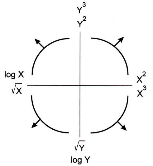
- Why? We're working with linear models. The more linear our data looks in terms of its features, the better we'll able to model the data.
fig
- Here, the bottom-left quadrant appears to match the shape of the scatter plot between
'horsepower'and'mpg'the best – let's try taking thelogof'horsepower'(the $x$ variable).
mpg['log hp'] = np.log(mpg['horsepower'])
- What does our data look like now?
px.scatter(mpg, x='log hp', y='mpg')
Predicting 'mpg' using log('horsepower')
- Let's fit another linear model.
car_model_log = LinearRegression()
car_model_log.fit(mpg[['log hp']], mpg['mpg'])
LinearRegression()In a Jupyter environment, please rerun this cell to show the HTML representation or trust the notebook.
On GitHub, the HTML representation is unable to render, please try loading this page with nbviewer.org.
LinearRegression()
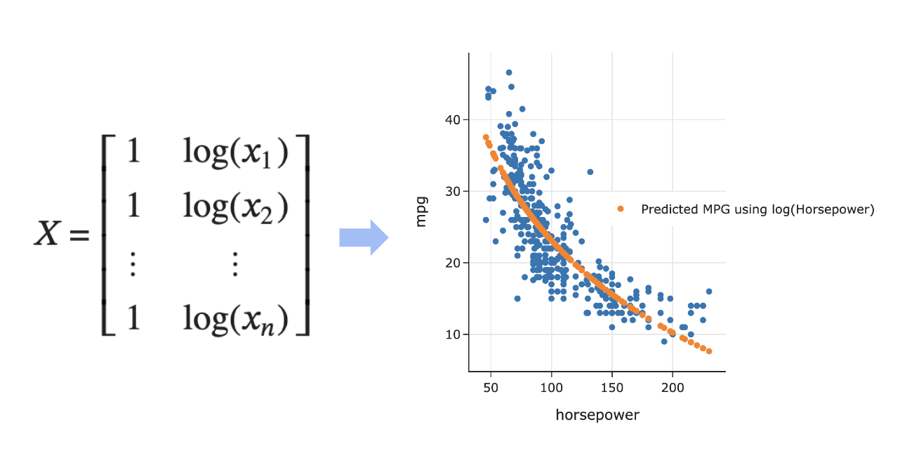
- Note that implicitly, we defined the following design matrix:
- What do our predictions look like now?
fig = px.scatter(mpg, x='log hp', y='mpg')
log_hp_points = pd.DataFrame({'log hp': [3.7, 5.5]})
fig = px.scatter(mpg, x='log hp', y='mpg')
fig.add_trace(go.Scatter(
    x=log_hp_points['log hp'],
    y=car_model_log.predict(log_hp_points),
    mode='lines',
    name='Predicted MPG using log(Horsepower)'
))
- The fit looks a bit better! How about the MSE?
# Using log hp:
mean_squared_error(mpg['mpg'], car_model_log.predict(mpg[['log hp']]))
20.152887978233167
# Using hp, from before:
mean_squared_error(mpg['mpg'], car_model.predict(mpg[['horsepower']]))
23.943662938603108
- Also a bit better!
- What do our predictions look like on the original, non-transformed scatter plot? Let's see:
fig = px.scatter(mpg, x='horsepower', y='mpg')
fig.add_trace(
    go.Scatter(
        x=mpg['horsepower'],
        y=car_model_log.intercept_ + car_model_log.coef_[0] * np.log(mpg['horsepower']),
        mode='markers', name='Predicted MPG using log(Horsepower)'
    )
)
fig
- Our predictions that used $\log(\text{Horsepower})$ as an input don't fall on a straight line. We shouldn't expect them to; the orange dots come from:
car_model_log.intercept_, car_model_log.coef_
(108.69970699574483, array([-18.58]))
Question 🤔 (Answer at practicaldsc.org/q)
Which hypothesis function is not linear in the parameters?
- A. $H(\vec{x}_i) = w_1 (x_i^{(1)} x_i^{(2)}) + \frac{w_2}{x_i^{(1)}} \sin \left( x_i^{(2)} \right)$
- B. $H(\vec{x}_i) = 2^{w_1} x_i^{(1)}$
- C. $H(\vec{x}_i) = \vec{w} \cdot \text{Aug}(\vec{x}_i)$
- D. $H(\vec{x}_i) = w_1 \cos (x_i^{(1)}) + w_2 2^{x_i^{(2)} \log x_i^{(3)}}$
- E. More than one of the above.
How do we fit hypothesis functions that aren't linear in the parameters?
- Suppose we want to fit the hypothesis function:
- This is not linear in terms of $w_0$ and $w_1$, so our results for linear regression don't apply.
- Possible solution: Try to transform the above equation so that it is linear in some other parameters, by applying an operation to both sides.
- See the attached Reference Slide for more details.
- Suppose we take the $\log$ of both sides of the equation.
- Then, using properties of logarithms, we have:
- Solution: Create a new hypothesis function, $T(x_i)$, with parameters $b_0$ and $b_1$, where $T(x_i) = b_0 + b_1 x_i$.
- This hypothesis function is related to $H(x_i)$ by the relationship $T(x_i) = \log H(x_i)$.
- $\vec{b}$ is related to $\vec{w}$ by $b_0 = \log w_0$ and $b_1 = w_1$.
- Our new observation vector, $\vec{z}$, is $\begin{bmatrix} \log y_1 \\ \log y_2 \\ ... \\ \log y_n \end{bmatrix}$.
- $T(x_i) = b_0 + b_1x_i$ is linear in its parameters, $b_0$ and $b_1$.
- Use the solution to the normal equations to find $\vec{b}^*$, and the relationship between $\vec{b}$ and $\vec{w}$ to find $\vec{w}^*$.
The modeling recipe, revisited
The original modeling recipe, from Lecture 11
- Choose a model.
- Choose a loss function.
- Minimize average loss (empirical risk) to find optimal model parameters, $\vec w^*$.
The updated modeling recipe
- Create, or engineer, features to best reflect the "meaning" behind data.
Recently, we've done this with one hot encoding and numerical-to-numerical transformations.
- Choose a model.
Recently, we've used the simple/multiple linear regression model.
- Choose a loss function.
Recently, we've mostly used squared loss.
- Minimize average loss (empirical risk) to find optimal model parameters, $\vec{w}^*$.
Originally, we had to use calculus or linear algebra to minimize empirical risk, but more recently we've just usedmodel.fit. This step is also called fitting the model to the data.
- Evaluate the performance of the model in relation to other models.
- We can do all of the above directly in
sklearn!
preprocessing and linear_models
- For the feature engineering step of the modeling pipeline, we will use
sklearn'spreprocessingmodule.
- For the model creation step of the modeling pipeline, we will use
sklearn'slinear_modelmodule, as we've already seen.linear_model.LinearRegressionis an example of an estimator class.
Transformer classes
- Transformers take in "raw" data and output "processed" data. They are used for creating features.
These are not directly related to "transformers" in large language models and neural networks.
- Transformers, like most relevant features of
sklearn, are classes, not functions, meaning you need to instantiate them and call their methods.
- Today, we'll introduce one transformer class,
StandardScaler. We'll look at how to write code to use it, and also discuss some of the underlying statistical nuances.
- Next class, we'll learn about another transformer class -
OneHotEncoder– and we'll see how to chain transformers and estimators together into larger Pipelines.
StandardScaler and standardized regression coefficients
Example: Predicting sales 📈
- To illustrate our first transformer class, we'll introduce a new dataset.
sales = pd.read_csv('data/sales.csv')
sales.head()
| net_sales | sq_ft | inventory | advertising | district_size | competing_stores | |
|---|---|---|---|---|---|---|
| 0 | 231.0 | 3.0 | 294 | 8.2 | 8.2 | 11 |
| 1 | 156.0 | 2.2 | 232 | 6.9 | 4.1 | 12 |
| 2 | 10.0 | 0.5 | 149 | 3.0 | 4.3 | 15 |
| 3 | 519.0 | 5.5 | 600 | 12.0 | 16.1 | 1 |
| 4 | 437.0 | 4.4 | 567 | 10.6 | 14.1 | 5 |
- For each of 26 stores, we have:
- net sales,
- square feet,
- inventory,
- advertising expenditure,
- district size, and
- number of competing stores.
- Our goal is to predict
'net_sales'as a function of other features.
An initial model
sales.head()
| net_sales | sq_ft | inventory | advertising | district_size | competing_stores | |
|---|---|---|---|---|---|---|
| 0 | 231.0 | 3.0 | 294 | 8.2 | 8.2 | 11 |
| 1 | 156.0 | 2.2 | 232 | 6.9 | 4.1 | 12 |
| 2 | 10.0 | 0.5 | 149 | 3.0 | 4.3 | 15 |
| 3 | 519.0 | 5.5 | 600 | 12.0 | 16.1 | 1 |
| 4 | 437.0 | 4.4 | 567 | 10.6 | 14.1 | 5 |
- No transformations are needed to predict
'net_sales'.
sales_model = LinearRegression()
sales_model.fit(X=sales.iloc[:, 1:], y=sales.iloc[:, 0])
LinearRegression()In a Jupyter environment, please rerun this cell to show the HTML representation or trust the notebook.
On GitHub, the HTML representation is unable to render, please try loading this page with nbviewer.org.
LinearRegression()
- Suppose we're interested in learning how the various features impact
'net_sales', rather than just predicting'net_sales'for a new store. We'd then look at the coefficients.
sales_model.coef_
array([16.2 , 0.17, 11.53, 13.58, -5.31])
coefs = pd.DataFrame().assign(
    column=sales.columns[1:],
    original_coef=sales_model.coef_,
).set_index('column')
coefs.plot(kind='barh', title='Original Coefficients')
- What do you notice?
sales.iloc[:, 1:]
| sq_ft | inventory | advertising | district_size | competing_stores | |
|---|---|---|---|---|---|
| 0 | 3.0 | 294 | 8.2 | 8.2 | 11 |
| 1 | 2.2 | 232 | 6.9 | 4.1 | 12 |
| 2 | 0.5 | 149 | 3.0 | 4.3 | 15 |
| ... | ... | ... | ... | ... | ... |
| 24 | 3.5 | 382 | 9.8 | 11.5 | 5 |
| 25 | 5.1 | 590 | 12.0 | 15.7 | 0 |
| 26 | 8.6 | 517 | 7.0 | 12.0 | 8 |
27 rows × 5 columns
Thought experiment
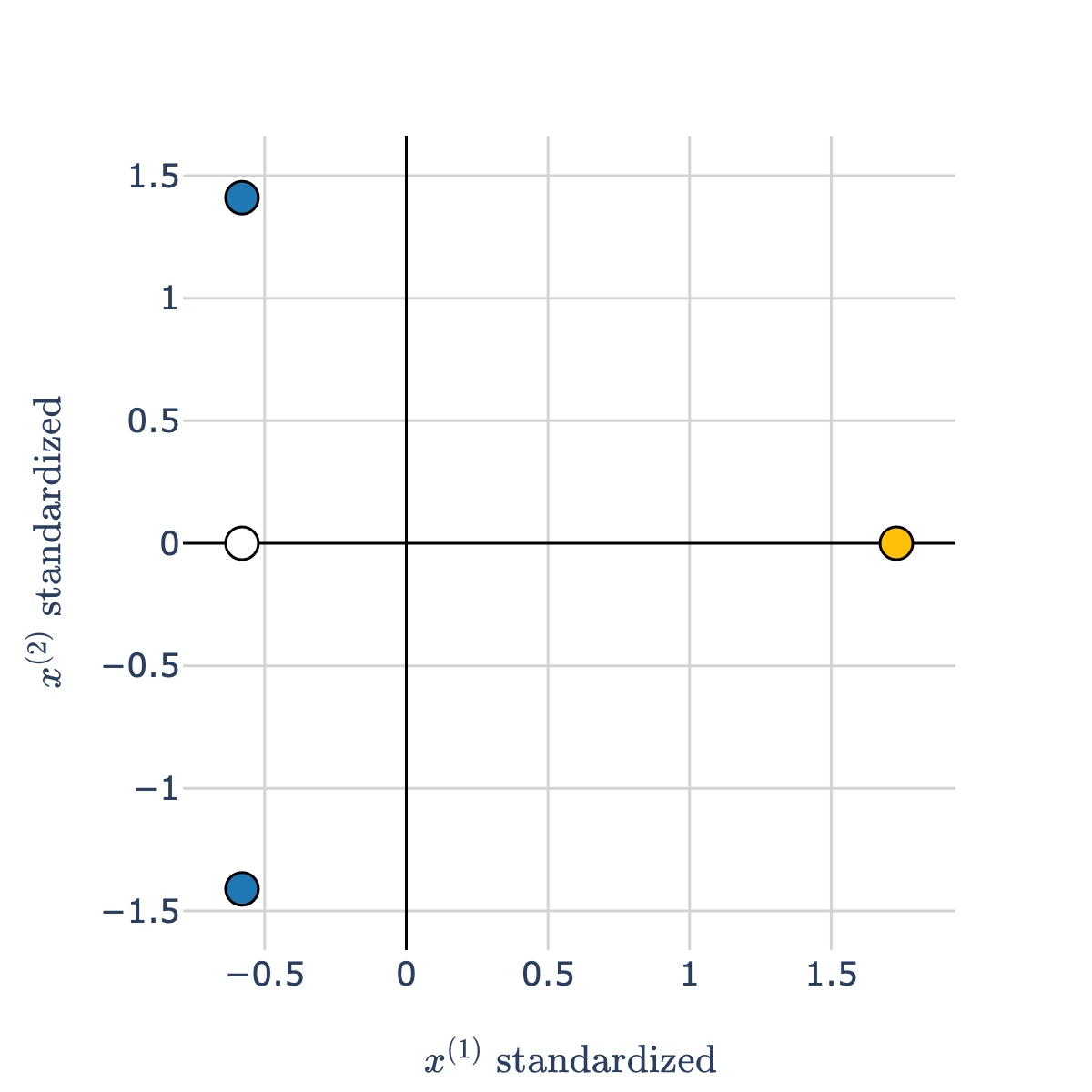
- Consider the white point in the scatter plot below.
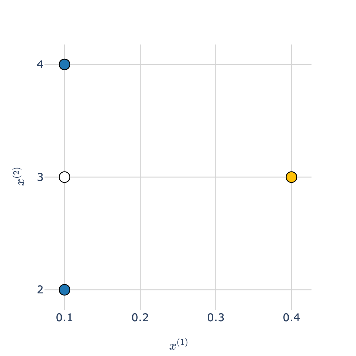
- Which class is it more "similar" to – blue or orange?
- Intuitively, the answer may be blue, but take a close look at the scale of the axes!
The orange point is much closer to the white point than the blue points are.
Standardization
- When we standardize two or more features, we bring them to the same scale.
- Recall: to standardize a feature $x_1, x_2, ..., x_n$, we use the formula: $$z(x_i) = \frac{x_i - \bar{x}}{\sigma_x}$$
Example: 1, 7, 7, 9.
- Mean: $\frac{1 + 7 + 7 + 9}{4} = \frac{24}{4} = 6$.
- Standard deviation:
$$\text{SD} = \sqrt{\frac{1}{4} \left( (1-6)^2 + (7-6)^2 + (7-6)^2 + (9-6)^2 \right)} = \sqrt{\frac{1}{4} \cdot 36} = 3$$
- Standardized data:
$$1 \mapsto \frac{1-6}{3} = \boxed{-\frac{5}{3}} \qquad 7 \mapsto \frac{7-6}{3} = \boxed{\frac{1}{3}} \qquad 7 \mapsto \boxed{\frac{1}{3}} \qquad 9 \mapsto \frac{9-6}{3} = \boxed{1}$$
Pre- and post- standardization
- Before we standardize both axes:
- After we standardize both axes:
- After we standardize, our features are measured on the same scales, so they can be compared directly.
Which features are most "important"?
- The most important feature is not necessarily the feature with largest magnitude coefficient, because different features may be on different scales.
But, it would be nice if the most important feature was the one with the largest magnitude coefficient!
coefs.plot(kind='barh', title='Original Coefficients')
sales.iloc[:, 1:]
| sq_ft | inventory | advertising | district_size | competing_stores | |
|---|---|---|---|---|---|
| 0 | 3.0 | 294 | 8.2 | 8.2 | 11 |
| 1 | 2.2 | 232 | 6.9 | 4.1 | 12 |
| 2 | 0.5 | 149 | 3.0 | 4.3 | 15 |
| ... | ... | ... | ... | ... | ... |
| 24 | 3.5 | 382 | 9.8 | 11.5 | 5 |
| 25 | 5.1 | 590 | 12.0 | 15.7 | 0 |
| 26 | 8.6 | 517 | 7.0 | 12.0 | 8 |
27 rows × 5 columns
- Here,
'inventory'values are much larger than'sq_ft'values, which means that the coefficient for'inventory'will inherently be smaller, even if'inventory'is a more important feature than'sq_ft'.
Intuition: if the values themselves are larger, you need to multiply them by smaller coefficients to get the same predictions!
- Solution: If you care about the interpretability of the resulting coefficients, standardize each feature before performing regression.
Example transformer: StandardScaler
StandardScalerstandardizes data using the mean and standard deviation of the data.
- First, we need to import the relevant class from
sklearn.preprocessing.
It's best practice to import just the relevant classes you need fromsklearn.
from sklearn.preprocessing import StandardScaler
- Like an estimator, we need to instantiate and fit our
OneHotEncoderinstsance before it can transform anything.
Here, "fitting" the transformer involves computing and saving the mean and SD of each column.
stdscaler = StandardScaler()
# Doesn't work! Need to fit first.
stdscaler.transform(sales.iloc[:, 1:])
---------------------------------------------------------------------------
NotFittedError                            Traceback (most recent call last)
Cell In[43], line 2
      1 # Doesn't work! Need to fit first.
----> 2 stdscaler.transform(sales.iloc[:, 1:])

File ~/miniforge3/envs/pds/lib/python3.10/site-packages/sklearn/utils/_set_output.py:313, in _wrap_method_output.<locals>.wrapped(self, X, *args, **kwargs)
    311 @wraps(f)
    312 def wrapped(self, X, *args, **kwargs):
--> 313     data_to_wrap = f(self, X, *args, **kwargs)
    314     if isinstance(data_to_wrap, tuple):
    315         # only wrap the first output for cross decomposition
    316         return_tuple = (
    317             _wrap_data_with_container(method, data_to_wrap[0], X, self),
    318             *data_to_wrap[1:],
    319         )

File ~/miniforge3/envs/pds/lib/python3.10/site-packages/sklearn/preprocessing/_data.py:1042, in StandardScaler.transform(self, X, copy)
   1027 def transform(self, X, copy=None):
   1028     """Perform standardization by centering and scaling.
   1029
   1030     Parameters
   (...)
   1040         Transformed array.
   1041     """
-> 1042     check_is_fitted(self)
   1044     copy = copy if copy is not None else self.copy
   1045     X = self._validate_data(
   1046         X,
   1047         reset=False,
   (...)
   1052         force_all_finite="allow-nan",
   1053     )

File ~/miniforge3/envs/pds/lib/python3.10/site-packages/sklearn/utils/validation.py:1661, in check_is_fitted(estimator, attributes, msg, all_or_any)
   1658     raise TypeError("%s is not an estimator instance." % (estimator))
   1660 if not _is_fitted(estimator, attributes, all_or_any):
-> 1661     raise NotFittedError(msg % {"name": type(estimator).__name__})

NotFittedError: This StandardScaler instance is not fitted yet. Call 'fit' with appropriate arguments before using this estimator.
# This is like saying "determine the mean and SD of each column in sales,
# other than the 'net_sales' column".
stdscaler.fit(sales.iloc[:, 1:])
StandardScaler()In a Jupyter environment, please rerun this cell to show the HTML representation or trust the notebook.
On GitHub, the HTML representation is unable to render, please try loading this page with nbviewer.org.
StandardScaler()
- Now, we can standardize any dataset, using the mean and standard deviation of the columns in
sales.iloc[:, 1:]. Typical usage is to fit transformer on a sample and use that already-fit transformer to transform future data.
stdscaler.transform([[5, 300, 10, 15, 6]])
array([[ 0.85, -0.47, 0.51, 1.05, -0.36]])
stdscaler.transform(sales.iloc[:, 1:].tail(5))
array([[-1.13, -1.31, -1.35, -1.6 ,  0.89],
       [ 0.14,  0.39,  0.4 ,  0.32, -0.36],
       [ 0.09, -0.03,  0.46,  0.36, -0.57],
       [ 0.9 ,  1.08,  1.05,  1.19, -1.61],
       [ 2.67,  0.69, -0.3 ,  0.46,  0.05]])
- We can peek under the hood and see what it computed!
stdscaler.mean_
array([ 3.33, 387.48, 8.1 , 9.69, 7.74])
stdscaler.var_
array([ 3.89, 35191.58, 13.72, 25.44, 23.08])
- If needed, the
fit_transformmethod will fit the transformer and then transform the data in one go.
new_scaler = StandardScaler()
new_scaler.fit_transform(sales.iloc[:, 1:].tail(5))
array([[-1.33, -1.79, -1.71, -1.88,  1.48],
       [-0.32,  0.28,  0.43,  0.19, -0.05],
       [-0.36, -0.24,  0.49,  0.23, -0.31],
       [ 0.29,  1.11,  1.22,  1.13, -1.58],
       [ 1.71,  0.64, -0.43,  0.34,  0.46]])
- Why are the values above different from the values in
stdscaler.transform(sales.iloc[:, 1:].tail(5))?
Interpreting standardized regression coefficients
- Now that we have a technique for standardizing the feature columns of
sales, let's fit a new regression object.
sales_model_std = LinearRegression()
sales_model_std.fit(X=stdscaler.transform(sales.iloc[:, 1:]),
                    y=sales.iloc[:, 0])
LinearRegression()In a Jupyter environment, please rerun this cell to show the HTML representation or trust the notebook.
On GitHub, the HTML representation is unable to render, please try loading this page with nbviewer.org.
LinearRegression()
- Let's now look at the resulting coefficients, and compare them to the coefficients before we standardized.
pd.DataFrame().assign(
    column=sales.columns[1:],
    original_coef=sales_model.coef_,
    standardized_coef=sales_model_std.coef_
).set_index('column').plot(kind='barh', barmode='group', title='Standardized and Original Coefficients')
- Did the performance of the resulting model change?
mean_squared_error(sales.iloc[:, 0],
                   sales_model.predict(sales.iloc[:, 1:]))
242.27445717154964
mean_squared_error(sales.iloc[:, 0],
                   sales_model_std.predict(stdscaler.transform(sales.iloc[:, 1:])))
242.27445717154956
- No!
The span of the design matrix did not change, so the predictions did not change. It's just the coefficients that changed.
Key takeaways
- The result of standardizing each feature (separately!) is that the units of each feature are on the same scale.
- There's no need to standardize the outcome (
'net_sales'here), since it's not being compared to anything. - Also, we can't standardize the column of all 1s.
- There's no need to standardize the outcome (
- Then, solve the normal equations. The resulting $w_0^*, w_1^*, \ldots, w_d^*$ are called the standardized regression coefficients.
- Standardized regression coefficients can be directly compared to one another.
Features with larger (absolute) standardized regression coefficients are most important to the model's predictions.
- As we saw on the previous slide, standardizing each feature does not change the MSE of the resulting hypothesis function!
StandardScaler summary
| Property | Example | Description |
|---|---|---|
| Initialize with parameters | stdscaler = StandardScaler() |
z-score the data (no parameters) |
| Fit the transformer | stdscaler.fit(X) |
Compute the mean and SD of X |
| Transform data in a dataset | feat = stdscaler.transform(X_new) |
z-score X_new with mean and SD of X |
| Fit and transform | stdscaler.fit_transform(X) |
Compute the mean and SD of X, then z-score X |
What's next?
- How does
OneHotEncoderwork?
- Even though we have a
StandardScalertransformer object, to actually use standardize our features AND make predictions, we need to:- Manually instantiate a
StandardScalerobject, and thenfitit. - Create a new design matrix by taking the result of calling
transformon theStandardScalerobject and concatenating other relevant numerical columns. - Manually instantiate a
LinearRegressionobject, and thenfitit using the result of the above step.
- Manually instantiate a
- As we build more and more sophisticated models, it will be challenging to keep track of all of these individual steps ourselves.
- As such, we often build Pipelines.