from lec_utils import *
def show_grouping_animation():
    src = "https://docs.google.com/presentation/d/1tBaFyHseIGsX5wmE3BdNLeVHnKksQtpzLhHge8Tzly0/embed?start=false&loop=false&delayms=60000&rm=minimal"
    width = 960
    height = 509
    display(IFrame(src, width, height))
Lecture 5
Aggregation: Grouping and Pivoting
EECS 398: Practical Data Science, Spring 2025
practicaldsc.org • github.com/practicaldsc/sp25 • 📣 See latest announcements here on Ed
YouTubeVideo('TLzUE-FyVcM')
Agenda 📆
- Introduction to the
groupbymethod. groupby's inner workings.- Advanced
groupbyusage. - Pivot tables using
pivot_table.
Remember to follow along in lecture by accessing the "blank" lecture notebook in our public GitHub repository.
And, read this guide, which describes how DataFrames work under the hood, and what to be careful of when working on homeworks.
Example: Palmer Penguins
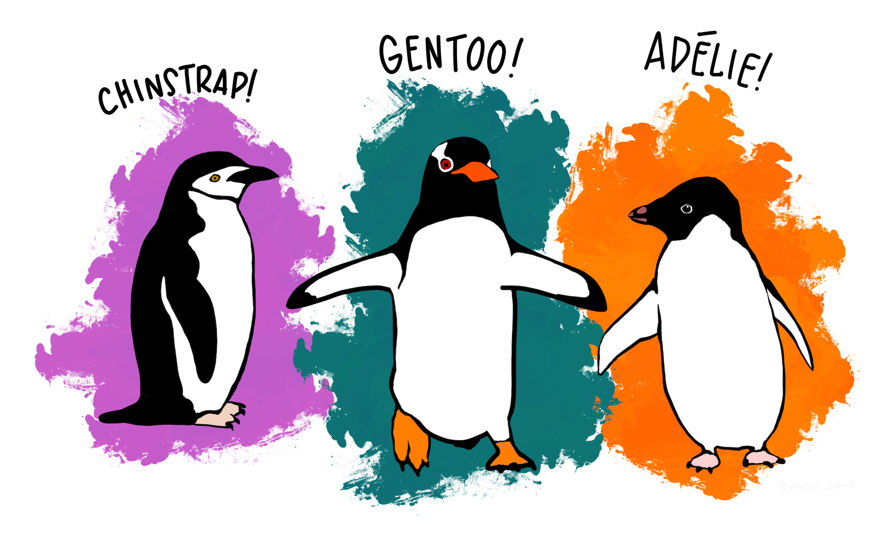 Artwork by @allison_horst
The dataset we'll work with for the rest of the lecture involves various measurements taken of three species of penguins in Antarctica.
IFrame('https://www.youtube-nocookie.com/embed/CCrNAHXUstU?si=-DntSyUNp5Kwitjm&start=11',
       width=560, height=315)
Loading the data
penguins = pd.read_csv('data/penguins.csv')
penguins
| species | island | bill_length_mm | bill_depth_mm | flipper_length_mm | body_mass_g | sex | |
|---|---|---|---|---|---|---|---|
| 0 | Adelie | Dream | 41.3 | 20.3 | 194.0 | 3550.0 | Male |
| 1 | Adelie | Torgersen | 38.5 | 17.9 | 190.0 | 3325.0 | Female |
| 2 | Adelie | Dream | 34.0 | 17.1 | 185.0 | 3400.0 | Female |
| ... | ... | ... | ... | ... | ... | ... | ... |
| 330 | Chinstrap | Dream | 46.6 | 17.8 | 193.0 | 3800.0 | Female |
| 331 | Adelie | Dream | 39.7 | 17.9 | 193.0 | 4250.0 | Male |
| 332 | Gentoo | Biscoe | 45.1 | 14.5 | 207.0 | 5050.0 | Female |
333 rows × 7 columns
- Here, each row corresponds to a single penguin, and each column corresponds to a different attribute (or feature) we have for each penguin.
- Data formatted in this way is sometimes called tidy data.
Visualizing the data
penguins.plot(kind='scatter',
              x='bill_length_mm',
              y='body_mass_g',
              color='species',
              title='Body Mass vs. Bill Length')
Aggregating
- Aggregating is the act of combining many values into a single value.
- Aggregations "hide" some of the detail in the data, and help understand bigger-picture trends.
- Example: What is the mean
'body_mass_g'for all penguins?
penguins['body_mass_g'].mean()
4207.057057057057
- Example: What is the mean
'body_mass_g'for each'species'?
A naïve approach to finding the mean 'body_mass_g' per 'species'
- First, we could identify all unique values in the
'species'column.
penguins['species'].unique()
array(['Adelie', 'Chinstrap', 'Gentoo'], dtype=object)
- Then, for each
'species', we could:- Query for just that
'species'. - Extract the
'body_mass_g'column and use themeanmethod on it.
- Query for just that
penguins.loc[penguins['species'] == 'Adelie', 'body_mass_g'].mean()
3706.1643835616437
penguins.loc[penguins['species'] == 'Chinstrap', 'body_mass_g'].mean()
3733.0882352941176
penguins.loc[penguins['species'] == 'Gentoo', 'body_mass_g'].mean()
5092.436974789916
- We could use a
for-loop, but remember, we want to avoid Pythonfor-loops.
The magic of groupby 🪄
- A better solution is to use the
groupbymethod.
# To find the overall mean 'body_mass_g':
penguins['body_mass_g'].mean()
4207.057057057057
# To find the mean 'body_mass_g' for each 'species':
penguins.groupby('species')['body_mass_g'].mean()
species
Adelie       3706.16
Chinstrap    3733.09
Gentoo       5092.44
Name: body_mass_g, dtype: float64
- Somehow, the
groupbymethod computes what we're looking for in just one line. How?
- We'll work through the internals, but remember this: if you need to calculate something for each group, use
groupby!
An illustrative example: Pets 🐱 🐶🐹
- Consider the DataFrame
pets, shown below.
| Species | Color | Weight | Age | |
|---|---|---|---|---|
| 0 | dog | black | 40 | 5.0 |
| 1 | cat | golden | 15 | 8.0 |
| 2 | cat | black | 20 | 9.0 |
| 3 | dog | white | 80 | 2.0 |
| 4 | dog | golden | 25 | 0.5 |
| 5 | hamster | golden | 1 | 3.0 |
- Let's see what happens under the hood when we use the
groupbymethod onpets.
show_grouping_animation()
"Split-apply-combine" paradigm
- The
groupbymethod involves three steps: split, apply, and combine.
This is the same terminology that thepandasdocumentation uses.
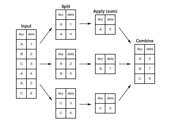
- Split breaks up and "groups" the rows of a DataFrame according to the specified key.
There is one "group" for every unique value of the key.
- Apply uses a function (e.g. aggregation, transformation, filtration) within the individual groups.
- Combine stitches the results of these operations into an output DataFrame.
- The split-apply-combine pattern can be parallelized to work on multiple computers or threads, by sending computations for each group to different processors.
Activity
Which penguin 'species' has the highest median 'bill_length_mm'?
penguins
| species | island | bill_length_mm | bill_depth_mm | flipper_length_mm | body_mass_g | sex | |
|---|---|---|---|---|---|---|---|
| 0 | Adelie | Dream | 41.3 | 20.3 | 194.0 | 3550.0 | Male |
| 1 | Adelie | Torgersen | 38.5 | 17.9 | 190.0 | 3325.0 | Female |
| 2 | Adelie | Dream | 34.0 | 17.1 | 185.0 | 3400.0 | Female |
| ... | ... | ... | ... | ... | ... | ... | ... |
| 330 | Chinstrap | Dream | 46.6 | 17.8 | 193.0 | 3800.0 | Female |
| 331 | Adelie | Dream | 39.7 | 17.9 | 193.0 | 4250.0 | Male |
| 332 | Gentoo | Biscoe | 45.1 | 14.5 | 207.0 | 5050.0 | Female |
333 rows × 7 columns
(
    penguins
    .groupby('species')
    ['bill_length_mm']
    .median()
    .idxmax()
)
'Chinstrap'
(
    penguins
    .groupby('species')
    ['bill_length_mm']
    .median()
    .plot(kind='barh', title='Median Bill Length of Each Species')
)
groupby's inner workings
How does groupby actually work?
- We've just evaluated a few expressions of the following form.
penguins.groupby('species')['bill_length_mm'].mean()
species
Adelie       38.82
Chinstrap    48.83
Gentoo       47.57
Name: bill_length_mm, dtype: float64
- There are three "building blocks"
in the above expression:
1. penguins.groupby('species').
First, we specify which column we want to group on.
1. ['bill_length_mm'].
Then, we select the other relevant columns for our calculations.
1. .mean().
Finally, we use an aggregation method.
- Let's see what each block contributes to the output.
DataFrameGroupBy objects
penguins.groupby('species')['bill_length_mm'].mean()
- If
dfis a DataFrame, thendf.groupby(key)returns aDataFrameGroupByobject.
This object represents the "split" in "split-apply-combine".
penguins.groupby('species')
<pandas.core.groupby.generic.DataFrameGroupBy object at 0x1529bd8d0>
# Creates one group for each unique value in the species column.
penguins.groupby('species').groups
{'Adelie': [0, 1, 2, 4, 6, 11, 12, 15, 19, 20, 21, 23, 25, 26, 33, 34, 36, 37, 38, 42, 49, 51, 52, 54, 59, 60, 61, 63, 64, 69, 70, 71, 77, 78, 79, 81, 85, 87, 90, 91, 94, 95, 96, 102, 103, 106, 107, 111, 112, 115, 117, 118, 120, 121, 123, 126, 127, 131, 133, 136, 139, 141, 143, 147, 150, 153, 158, 160, 164, 165, 167, 168, 172, 173, 174, 177, 178, 184, 188, 193, 198, 201, 203, 207, 208, 210, 214, 216, 217, 218, 219, 220, 223, 227, 228, 229, 230, 232, 234, 237, ...], 'Chinstrap': [3, 5, 7, 8, 13, 18, 22, 24, 28, 30, 31, 39, 48, 50, 55, 58, 74, 84, 92, 93, 97, 99, 101, 105, 110, 125, 128, 130, 135, 140, 142, 146, 152, 162, 163, 176, 180, 183, 187, 190, 192, 195, 197, 206, 209, 211, 224, 235, 240, 241, 242, 246, 251, 260, 261, 265, 266, 271, 282, 302, 308, 311, 312, 317, 327, 328, 329, 330], 'Gentoo': [9, 10, 14, 16, 17, 27, 29, 32, 35, 40, 41, 43, 44, 45, 46, 47, 53, 56, 57, 62, 65, 66, 67, 68, 72, 73, 75, 76, 80, 82, 83, 86, 88, 89, 98, 100, 104, 108, 109, 113, 114, 116, 119, 122, 124, 129, 132, 134, 137, 138, 144, 145, 148, 149, 151, 154, 155, 156, 157, 159, 161, 166, 169, 170, 171, 175, 179, 181, 182, 185, 186, 189, 191, 194, 196, 199, 200, 202, 204, 205, 212, 213, 215, 221, 222, 225, 226, 231, 233, 236, 245, 247, 248, 252, 253, 257, 264, 267, 268, 275, ...]}
DataFrameGroupByobjects have agroupsattribute, which is a dictionary in which the keys are group names and the values are lists of row labels.
We won't actually use this, but it's helpful in understanding howgroupbyworks under-the-hood.
Column extraction
penguins.groupby('species')['bill_length_mm'].mean()
- After creating a
DataFrameGroupByobject, we typically select the relevant column(s) that we want to aggregate.
If we don't, we may run into errors if trying to use a numeric aggregation method on non-numeric columns, as we saw earlier.
Also, this is more efficient, since the aggregations are only performed on the columns you care about, rather than all columns.
- The result is either a
SeriesGroupByorDataFrameGroupByobject, depending on what's passed in.
penguins.groupby('species')['bill_length_mm']
<pandas.core.groupby.generic.SeriesGroupBy object at 0x152a39330>
penguins.groupby('species')[['bill_length_mm', 'bill_depth_mm']]
<pandas.core.groupby.generic.DataFrameGroupBy object at 0x152a3a650>
Aggregation
penguins.groupby('species')['bill_length_mm'].mean()
- Once we create a
DataFrameGroupByorSeriesGroupByobject, we need to apply some function separately to each group, and combine the results.
- The most common operation we apply to each group is an aggregation, but we'll see examples of filtrations and transformations soon.
Remember, aggregation is the act of combining many values into a single value.
- To perform an aggregation, use an aggregation method on the
DataFrameGroupByorSeriesGroupByobject, e.g..mean(),.max(), or.median().
Let's look at some examples.
# Note that this worked on the entire DataFrame!
# But, if all we wanted are the sums of `'body_mass_g'
# for each species, this is slower than
# penguins.groupby('species')['body_mass_g'].sum().
penguins.groupby('species').sum()
| island | bill_length_mm | bill_depth_mm | flipper_length_mm | body_mass_g | sex | |
|---|---|---|---|---|---|---|
| species | ||||||
| Adelie | DreamTorgersenDreamBiscoeTorgersenBiscoeTorger... | 5668.3 | 2678.7 | 27755.0 | 541100.0 | MaleFemaleFemaleMaleFemaleMaleFemaleMaleFemale... |
| Chinstrap | DreamDreamDreamDreamDreamDreamDreamDreamDreamD... | 3320.7 | 1252.6 | 13316.0 | 253850.0 | FemaleFemaleMaleMaleFemaleFemaleFemaleFemaleFe... |
| Gentoo | BiscoeBiscoeBiscoeBiscoeBiscoeBiscoeBiscoeBisc... | 5660.6 | 1784.6 | 25851.0 | 606000.0 | FemaleFemaleFemaleFemaleMaleFemaleFemaleMaleMa... |
# Often used in conjunction with sort_values.
# Remember this when you work on the activity in a few slides!
penguins.groupby('species').last()
| island | bill_length_mm | bill_depth_mm | flipper_length_mm | body_mass_g | sex | |
|---|---|---|---|---|---|---|
| species | ||||||
| Adelie | Dream | 39.7 | 17.9 | 193.0 | 4250.0 | Male |
| Chinstrap | Dream | 46.6 | 17.8 | 193.0 | 3800.0 | Female |
| Gentoo | Biscoe | 45.1 | 14.5 | 207.0 | 5050.0 | Female |
# Similar to value_counts, but not identical!
penguins.groupby('species').size()
species
Adelie       146
Chinstrap     68
Gentoo       119
dtype: int64
penguins['species'].value_counts()
species
Adelie       146
Gentoo       119
Chinstrap     68
Name: count, dtype: int64
Reminder: Column independence
- As we've seen, within each group, the aggregation method is applied to each column independently.
penguins.groupby('species').max()
| island | bill_length_mm | bill_depth_mm | flipper_length_mm | body_mass_g | sex | |
|---|---|---|---|---|---|---|
| species | ||||||
| Adelie | Torgersen | 46.0 | 21.5 | 210.0 | 4775.0 | Male |
| Chinstrap | Dream | 58.0 | 20.8 | 212.0 | 4800.0 | Male |
| Gentoo | Biscoe | 59.6 | 17.3 | 231.0 | 6300.0 | Male |
- The above result is not telling us that there is a
'Adelie'penguin with a'body_mass_g'of4775.0that lived on'Torgersen'island.
# This penguin lived on Biscoe island!
penguins.loc[(penguins['species'] == 'Adelie') & (penguins['body_mass_g'] == 4775.0)]
| species | island | bill_length_mm | bill_depth_mm | flipper_length_mm | body_mass_g | sex | |
|---|---|---|---|---|---|---|---|
| 255 | Adelie | Biscoe | 43.2 | 19.0 | 197.0 | 4775.0 | Male |
Activity
Find the 'species', 'island', and 'body_mass_g' of the heaviest 'Male' and 'Female' penguins in penguins.
# General idea: Sort the penguibs by mass in decreasing order.
# Then, the first male penguin that appears is the heaviest male penguin,
# and the first female penguin that appears is the heaviest female penguin.
# For each sex, take the first row.
(
    penguins
    .sort_values('body_mass_g', ascending=False)
    .groupby('sex')
    .first()
)
| species | island | bill_length_mm | bill_depth_mm | flipper_length_mm | body_mass_g | |
|---|---|---|---|---|---|---|
| sex | ||||||
| Female | Gentoo | Biscoe | 45.2 | 14.8 | 212.0 | 5200.0 |
| Male | Gentoo | Biscoe | 49.2 | 15.2 | 221.0 | 6300.0 |
Activity
What proportion of penguins of each 'species' live on 'Dream' island?
*Hint*: If you've read the guide, this activity will be much easier!
(
    penguins
    .assign(is_Dream=penguins['island'] == 'Dream')
    .groupby('species')
    ['is_Dream']
    .mean()
)
species
Adelie       0.38
Chinstrap    1.00
Gentoo       0.00
Name: is_Dream, dtype: float64
Advanced groupby usage
Beyond default aggregation methods
- There are many built-in aggregation methods, like
.mean(),.max(), and.last().
- What if the aggregation method you want to use doesn't already exist in
pandas, or what if you want to apply different aggregation methods to different columns?
- Or, what if you don't want to perform an aggregation, but want to perform some other operation separately on each group?
Grouping method 1: agg
After grouping, use the
aggmethod if you want to aggregate with:- A single function (either built-in or one that you define!).
- A list of functions.
- A dictionary mapping column names to functions.
Refer to the documentation for a comprehensive list.
Per the documentation,aggis an alias foraggregate.
- Example: How many penguins are there of each
'species', and what is the mean'body_mass_g'of each'species'?
(
    penguins
    .groupby('species')
    ['body_mass_g']
    .agg(['count', 'mean'])
)
| count | mean | |
|---|---|---|
| species | ||
| Adelie | 146 | 3706.16 |
| Chinstrap | 68 | 3733.09 |
| Gentoo | 119 | 5092.44 |
- Note that we call
agga "grouping method" because it comes after a call togroupby.
agg with different aggregation methods for different columns
- Example: What is the maximum
'bill_length_mm'of each'species', and which'island's is each'species'found on?
(
    penguins
    .groupby('species')
    .aggregate({'bill_length_mm': 'max', 'island': 'unique'})
)
| bill_length_mm | island | |
|---|---|---|
| species | ||
| Adelie | 46.0 | [Dream, Torgersen, Biscoe] |
| Chinstrap | 58.0 | [Dream] |
| Gentoo | 59.6 | [Biscoe] |
agg with a custom aggregation method
- Example: What is the second largest recorded
'body_mass_g'for each'species'?
# Here, the argument to agg is a function,
# which takes in a Series and returns a scalar.
def second_largest(s):
    return s.sort_values().iloc[-2]
(
    penguins
    .groupby('species')
    ['body_mass_g']
    .agg(second_largest)
)
species
Adelie       4725.0
Chinstrap    4550.0
Gentoo       6050.0
Name: body_mass_g, dtype: float64
- Key idea: If you give
agga custom function, it should map $\texttt{Series} \rightarrow \texttt{number}$.
Grouping method 2: filter
- As we saw last class, a query keeps rows that satisfy conditions.
For instance, to see the individual penguins with a'bill_length_mm'over 47 mm:
# This is a query, NOT a filter for the purposes of this slide.
penguins[penguins['bill_length_mm'] > 47]
| species | island | bill_length_mm | bill_depth_mm | flipper_length_mm | body_mass_g | sex | |
|---|---|---|---|---|---|---|---|
| 5 | Chinstrap | Dream | 50.1 | 17.9 | 190.0 | 3400.0 | Female |
| 7 | Chinstrap | Dream | 51.4 | 19.0 | 201.0 | 3950.0 | Male |
| 8 | Chinstrap | Dream | 51.3 | 19.2 | 193.0 | 3650.0 | Male |
| ... | ... | ... | ... | ... | ... | ... | ... |
| 327 | Chinstrap | Dream | 49.3 | 19.9 | 203.0 | 4050.0 | Male |
| 328 | Chinstrap | Dream | 50.7 | 19.7 | 203.0 | 4050.0 | Male |
| 329 | Chinstrap | Dream | 51.3 | 19.9 | 198.0 | 3700.0 | Male |
106 rows × 7 columns
- A filter, on the other hand, keeps entire groups that satisfy conditions.
- For instance, to see the penguin
'species'with an average'bill_length_mm'over 47 mm, use thefiltermethod aftergroupby:
(
    penguins
    .groupby('species')
    .filter(lambda df: df['bill_length_mm'].mean() > 47)
)
| species | island | bill_length_mm | bill_depth_mm | flipper_length_mm | body_mass_g | sex | |
|---|---|---|---|---|---|---|---|
| 3 | Chinstrap | Dream | 45.5 | 17.0 | 196.0 | 3500.0 | Female |
| 5 | Chinstrap | Dream | 50.1 | 17.9 | 190.0 | 3400.0 | Female |
| 7 | Chinstrap | Dream | 51.4 | 19.0 | 201.0 | 3950.0 | Male |
| ... | ... | ... | ... | ... | ... | ... | ... |
| 329 | Chinstrap | Dream | 51.3 | 19.9 | 198.0 | 3700.0 | Male |
| 330 | Chinstrap | Dream | 46.6 | 17.8 | 193.0 | 3800.0 | Female |
| 332 | Gentoo | Biscoe | 45.1 | 14.5 | 207.0 | 5050.0 | Female |
187 rows × 7 columns
- Notice that the above DataFrame has 187 rows, fewer than the 333 in the full DataFrame. That's because there are no
'Adelie'penguins above!
# Since 'Adelie's have a mean 'bill_length_mm' below 47, they aren't included in the output above.
penguins.groupby('species')['bill_length_mm'].mean()
species
Adelie       38.82
Chinstrap    48.83
Gentoo       47.57
Name: bill_length_mm, dtype: float64
- Key idea: If you give
filtera custom function, it should map $\texttt{DataFrame} \rightarrow \texttt{Boolean}$. The resulting DataFrame will only have the groups for which the custom function returnedTrue.
Activity
There is only one penguins 'species' with:
- At least 100 penguins.
- At least 60
'Female'penguins.
Find the 'species' using a single expression (i.e. no intermediate variables). Use filter.
(
    penguins
    .groupby('species')
    .filter(lambda df: (df.shape[0] >= 100) and ((df['sex'] == 'Female').sum() >= 60))
    ['species']
    .unique()
    [0]
)
'Adelie'
# Note that to just find the 'species' with at least 100 penguins,
# we didn't need to group:
penguins['species'].value_counts()
species
Adelie       146
Gentoo       119
Chinstrap     68
Name: count, dtype: int64
penguins.loc[penguins['sex'] == 'Female', 'species'].value_counts()
species
Adelie       73
Gentoo       58
Chinstrap    34
Name: count, dtype: int64
Grouping method 3: transform
- Use the
transformgrouping method if you want to apply a function separately to each group.
- Example: How much heavier is each penguin than the average penguin of their
'species'?
penguins.groupby('species')['body_mass_g'].transform(lambda s: s - s.mean())
0     -156.16
1     -381.16
2     -306.16
        ...
330     66.91
331    543.84
332    -42.44
Name: body_mass_g, Length: 333, dtype: float64
penguins['body_mass_g']
0      3550.0
1      3325.0
2      3400.0
        ...
330    3800.0
331    4250.0
332    5050.0
Name: body_mass_g, Length: 333, dtype: float64
- Notice that penguin 332's transformed
'body_mass_g'is negative, even though their actual'body_mass_g'is very large; this is because they have a below-average'body_mass_g'for their'species'.
- Key idea: If you give
transforma custom function, it should map $\texttt{Series} \rightarrow \texttt{Series}$.
Grouping method 4: apply
- Sometimes, you want to apply an operation separately for each group, but the operation isn't possible using
agg,filter, ortransform.
- The
applygrouping method is like a swiss-army knife.
It can do anythingaggortransformcan do, and more.
Only use it if necessary, because it's slower thanaggandtransform!
- Example: Find the two heaviest penguins per
'species'.
penguins.groupby('species').apply(lambda df: df.sort_values('body_mass_g', ascending=False).head(2))
| species | island | bill_length_mm | bill_depth_mm | flipper_length_mm | body_mass_g | sex | ||
|---|---|---|---|---|---|---|---|---|
| species | ||||||||
| Adelie | 255 | Adelie | Biscoe | 43.2 | 19.0 | 197.0 | 4775.0 | Male |
| 174 | Adelie | Biscoe | 41.0 | 20.0 | 203.0 | 4725.0 | Male | |
| Chinstrap | 99 | Chinstrap | Dream | 52.0 | 20.7 | 210.0 | 4800.0 | Male |
| 187 | Chinstrap | Dream | 52.8 | 20.0 | 205.0 | 4550.0 | Male | |
| Gentoo | 268 | Gentoo | Biscoe | 49.2 | 15.2 | 221.0 | 6300.0 | Male |
| 189 | Gentoo | Biscoe | 59.6 | 17.0 | 230.0 | 6050.0 | Male |
- Example: Find the
'flipper_length_mm'of the heaviest penguin of each'species'.
(
    penguins
    .groupby('species')
    .apply(
        lambda df: df.sort_values('body_mass_g', ascending=False)['flipper_length_mm'].iloc[0]
    )
)
species
Adelie       197.0
Chinstrap    210.0
Gentoo       221.0
dtype: float64
- Key idea: If you give
applya custom function, it should map $\texttt{DataFrame} \rightarrow \texttt{anything}$. The outputs of the custom function will be stitched together intelligently bypandas.
⭐️ The grouping method cheat sheet: agg, filter, transform, and apply ⭐️
After grouping, use:
- The
aggmethod if you want to aggregate values, separately for each group.
If you giveagga custom function, it should map $\texttt{Series} \rightarrow \texttt{number}$.
penguins.groupby('species')['body_mass_g'].agg(lambda s: s.sort_values().iloc[-2])
species
Adelie       4725.0
Chinstrap    4550.0
Gentoo       6050.0
Name: body_mass_g, dtype: float64
- The
filtermethod if you want to keep groups that satisfy certain conditions.
If you givefiltera custom function, it should map $\texttt{DataFrame} \rightarrow \texttt{Boolean}$. The resulting DataFrame will only have the groups for which the custom function returnedTrue.
(
    penguins
    .groupby('species')
    .filter(lambda df: (df.shape[0] >= 100) and ((df['sex'] == 'Female').sum() >= 60))
)
| species | island | bill_length_mm | bill_depth_mm | flipper_length_mm | body_mass_g | sex | |
|---|---|---|---|---|---|---|---|
| 0 | Adelie | Dream | 41.3 | 20.3 | 194.0 | 3550.0 | Male |
| 1 | Adelie | Torgersen | 38.5 | 17.9 | 190.0 | 3325.0 | Female |
| 2 | Adelie | Dream | 34.0 | 17.1 | 185.0 | 3400.0 | Female |
| ... | ... | ... | ... | ... | ... | ... | ... |
| 325 | Adelie | Torgersen | 35.2 | 15.9 | 186.0 | 3050.0 | Female |
| 326 | Adelie | Dream | 41.1 | 18.1 | 205.0 | 4300.0 | Male |
| 331 | Adelie | Dream | 39.7 | 17.9 | 193.0 | 4250.0 | Male |
146 rows × 7 columns
- The
transformmethod if you want to modify the values within each group separately.
If you givetransforma custom function, it should map $\texttt{Series} \rightarrow \texttt{Series}$.
penguins.groupby('species')['body_mass_g'].transform(lambda s: s - s.mean())
0     -156.16
1     -381.16
2     -306.16
        ...
330     66.91
331    543.84
332    -42.44
Name: body_mass_g, Length: 333, dtype: float64
- The
applymethod if you want to perform some general operation on each group separately.
If you giveapplya custom function, it should map $\texttt{DataFrame} \rightarrow \texttt{anything}$.
penguins.groupby('species').apply(lambda df: df.sort_values('body_mass_g', ascending=False).head(2))
| species | island | bill_length_mm | bill_depth_mm | flipper_length_mm | body_mass_g | sex | ||
|---|---|---|---|---|---|---|---|---|
| species | ||||||||
| Adelie | 255 | Adelie | Biscoe | 43.2 | 19.0 | 197.0 | 4775.0 | Male |
| 174 | Adelie | Biscoe | 41.0 | 20.0 | 203.0 | 4725.0 | Male | |
| Chinstrap | 99 | Chinstrap | Dream | 52.0 | 20.7 | 210.0 | 4800.0 | Male |
| 187 | Chinstrap | Dream | 52.8 | 20.0 | 205.0 | 4550.0 | Male | |
| Gentoo | 268 | Gentoo | Biscoe | 49.2 | 15.2 | 221.0 | 6300.0 | Male |
| 189 | Gentoo | Biscoe | 59.6 | 17.0 | 230.0 | 6050.0 | Male |
Grouping with multiple columns
- When we group with multiple columns, one group is created for every unique combination of elements in the specified columns.
In the output below, why are there only 5 rows, rather than $3 \times 3 = 9$ rows, when there are 3 unique'species'and 3 unique'island's?
# Read this as:
species_and_island = (
    penguins.groupby(['species', 'island'])         # for every combination of 'species' and 'island' in the DataFrame,
    [['bill_length_mm', 'bill_depth_mm']].mean()    # calculate the mean 'bill_length_mm' and the mean 'bill_depth_mm'.
)
species_and_island
| bill_length_mm | bill_depth_mm | ||
|---|---|---|---|
| species | island | ||
| Adelie | Biscoe | 38.98 | 18.37 |
| Dream | 38.52 | 18.24 | |
| Torgersen | 39.04 | 18.45 | |
| Chinstrap | Dream | 48.83 | 18.42 |
| Gentoo | Biscoe | 47.57 | 15.00 |
- Advice: When grouping on multiple columns, the result usually has a
MultiIndex; usereset_indexor setas_index=Falseingroupbyto avoid this.
# Now, this looks like a regular DataFrame!
species_and_island.reset_index()
| species | island | bill_length_mm | bill_depth_mm | |
|---|---|---|---|---|
| 0 | Adelie | Biscoe | 38.98 | 18.37 |
| 1 | Adelie | Dream | 38.52 | 18.24 |
| 2 | Adelie | Torgersen | 39.04 | 18.45 |
| 3 | Chinstrap | Dream | 48.83 | 18.42 |
| 4 | Gentoo | Biscoe | 47.57 | 15.00 |
Pivot tables using pivot_table
Pivot tables: An extension of grouping
- Pivot tables are a compact way to display tables for humans to read.
| sex | Female | Male |
|---|---|---|
| species | ||
| Adelie | 3368.84 | 4043.49 |
| Chinstrap | 3527.21 | 3938.97 |
| Gentoo | 4679.74 | 5484.84 |
- Notice that each value in the table is the average of
'body_mass_g'of penguins, for every combination of'species'and'sex'.
- You can think of pivot tables as grouping using two columns, then "pivoting" one of the group labels into columns.
pivot_table
- The
pivot_tableDataFrame method aggregates a DataFrame using two columns. To use it:
df.pivot_table(index=index_col,
                       columns=columns_col,
                       values=values_col,
                       aggfunc=func)
- The resulting DataFrame will have:
- One row for every unique value in
index_col. - One column for every unique value in
columns_col. - Values determined by applying
funcon values invalues_col.
- One row for every unique value in
- Example: Find the average
'body_mass_g'for every combination of'species'and'sex'.
penguins.pivot_table(
    index='species',
    columns='sex',
    values='body_mass_g',
    aggfunc='mean'
)
| sex | Female | Male |
|---|---|---|
| species | ||
| Adelie | 3368.84 | 4043.49 |
| Chinstrap | 3527.21 | 3938.97 |
| Gentoo | 4679.74 | 5484.84 |
# Same information as above, but harder to read!
(
    penguins
    .groupby(['species', 'sex'])
    [['body_mass_g']]
    .mean()
)
| body_mass_g | ||
|---|---|---|
| species | sex | |
| Adelie | Female | 3368.84 |
| Male | 4043.49 | |
| Chinstrap | Female | 3527.21 |
| Male | 3938.97 | |
| Gentoo | Female | 4679.74 |
| Male | 5484.84 |
Example: Finding the number of penguins per 'island' and 'species'
penguins
| species | island | bill_length_mm | bill_depth_mm | flipper_length_mm | body_mass_g | sex | |
|---|---|---|---|---|---|---|---|
| 0 | Adelie | Dream | 41.3 | 20.3 | 194.0 | 3550.0 | Male |
| 1 | Adelie | Torgersen | 38.5 | 17.9 | 190.0 | 3325.0 | Female |
| 2 | Adelie | Dream | 34.0 | 17.1 | 185.0 | 3400.0 | Female |
| ... | ... | ... | ... | ... | ... | ... | ... |
| 330 | Chinstrap | Dream | 46.6 | 17.8 | 193.0 | 3800.0 | Female |
| 331 | Adelie | Dream | 39.7 | 17.9 | 193.0 | 4250.0 | Male |
| 332 | Gentoo | Biscoe | 45.1 | 14.5 | 207.0 | 5050.0 | Female |
333 rows × 7 columns
- Suppose we want to find the number of penguins in
penguinsper'island'and'species'. We can do so withoutpivot_table:
penguins.value_counts(['island', 'species'])
island     species
Biscoe     Gentoo       119
Dream      Chinstrap     68
           Adelie        55
Torgersen  Adelie        47
Biscoe     Adelie        44
Name: count, dtype: int64
penguins.groupby(['island', 'species']).size()
island     species
Biscoe     Adelie        44
           Gentoo       119
Dream      Adelie        55
           Chinstrap     68
Torgersen  Adelie        47
dtype: int64
- But the data is arguably easier to interpret when we do use
pivot_table:
penguins.pivot_table(
    index='species',
    columns='island',
    values='bill_length_mm', # Choice of column here doesn't actually matter! Why?
    aggfunc='count',
)
| island | Biscoe | Dream | Torgersen |
|---|---|---|---|
| species | |||
| Adelie | 44.0 | 55.0 | 47.0 |
| Chinstrap | NaN | 68.0 | NaN |
| Gentoo | 119.0 | NaN | NaN |
- Note that there is a
NaNat the intersection of'Biscoe'and'Chinstrap', because there were no Chinstrap penguins on Biscoe Island.NaNstands for "not a number." It isnumpyandpandas' version of a null value (the regular Python null value isNone). We'll learn more about how to deal with these soon.
- We can either use the
fillnamethod afterwards or thefill_valueargument to fill inNaNs.
penguins.pivot_table(
    index='species',
    columns='island',
    values='bill_length_mm',
    aggfunc='count',
    fill_value=0,
)
| island | Biscoe | Dream | Torgersen |
|---|---|---|---|
| species | |||
| Adelie | 44 | 55 | 47 |
| Chinstrap | 0 | 68 | 0 |
| Gentoo | 119 | 0 | 0 |
Granularity
- Each row of the original
penguinsDataFrame represented a single penguin, and each column represented features of the penguins.
penguins
| species | island | bill_length_mm | bill_depth_mm | flipper_length_mm | body_mass_g | sex | |
|---|---|---|---|---|---|---|---|
| 0 | Adelie | Dream | 41.3 | 20.3 | 194.0 | 3550.0 | Male |
| 1 | Adelie | Torgersen | 38.5 | 17.9 | 190.0 | 3325.0 | Female |
| 2 | Adelie | Dream | 34.0 | 17.1 | 185.0 | 3400.0 | Female |
| ... | ... | ... | ... | ... | ... | ... | ... |
| 330 | Chinstrap | Dream | 46.6 | 17.8 | 193.0 | 3800.0 | Female |
| 331 | Adelie | Dream | 39.7 | 17.9 | 193.0 | 4250.0 | Male |
| 332 | Gentoo | Biscoe | 45.1 | 14.5 | 207.0 | 5050.0 | Female |
333 rows × 7 columns
- What is the granularity of the DataFrame below?
That is, what does each row represent?
penguins.pivot_table(
    index='species',
    columns='island',
    values='bill_length_mm',
    aggfunc='count',
    fill_value=0,
)
| island | Biscoe | Dream | Torgersen |
|---|---|---|---|
| species | |||
| Adelie | 44 | 55 | 47 |
| Chinstrap | 0 | 68 | 0 |
| Gentoo | 119 | 0 | 0 |
Reshaping
pivot_tablereshapes DataFrames from "long" to "wide".
- Other DataFrame reshaping methods:
melt: Un-pivots a DataFrame. Very useful in data cleaning.pivot: Likepivot_table, but doesn't do aggregation.stack: Pivots multi-level columns to multi-indices.unstack: Pivots multi-indices to columns.
- Google, the documentation, and ChatGPT are your friends!