# Run this cell to get everything set up.
from lec_utils import *
import lec24_util as util

diabetes = pd.read_csv('data/diabetes.csv')

from sklearn.model_selection import train_test_split
diabetes = diabetes[(diabetes['Glucose'] > 0) & (diabetes['BMI'] > 0)]
X_train, X_test, y_train, y_test = (
    train_test_split(diabetes[['Glucose', 'BMI']], diabetes['Outcome'], random_state=11)
)

from ipywidgets import interact

import warnings
warnings.simplefilter('ignore')

Lecture 24

Logistic Regression

EECS 398-003: Practical Data Science, Fall 2024

practicaldsc.org • github.com/practicaldsc/fa24

Announcements 📣

• The Portfolio Homework's checkpoint is due on Monday, November 25th – no slip days allowed!
  The full homework is due on Saturday, December 7th (no slip days!).

• Homework 10 is (finally!) out, and is due on Monday, December 2nd.
  Plan to finish it earlier, since we won't be able to offer much help over Thanksgiving.
  There will still be a Homework 11, but it'll be max 3 questions.

• Consider entering the Big Ten Data Viz Championship. Submissions are due on January 15th. Read more here.
  Help Michigan defend its title!

• Enrollment begins today. Some suggested courses for next semester can be found in #306 on Ed.
  And please help spread the word about 398!

Agenda

• Recap: Classification techniques and classifier evaluation.
• Predicting probabilities.
• Cross-entropy loss.
• From probabilities to decisions.

Question 🤔 (Answer at practicaldsc.org/q)

Remember that you can always ask questions anonymously at the link above!

Recap: Classification techniques and classifier evaluation

---

Classification

• A regression problem is one in which we're given a feature vector $\vec{x}$ and need to predict a real-valued target variable, $y$.
  Example: Given today's temperature, precipitation, and wind chill, what will tomorrow's high temperature be?

• A classification problem is one in which we're given a feature vector $\vec{x}$ and need to predict a categorical target variable, $y$.
  Example: Given today's temperature, precipitation, and wind chill, will it snow tomorrow?

• In binary classification, there are only two possible values of the target variable (typically 1 and 0); in multi-class classification, there can be more than two possible values of the target variable.

• Last class, we learned about two classification techniques:
  • $k$-Nearest Neighbors 🏡🏠.
  • Decision trees 🎄.

Accuracy of COVID tests

• The results of 100 Michigan Medicine COVID tests are given below.

	Predicted Negative	Predicted Positive
Actually Negative	TN = 90 ✅	FP = 1 ❌
Actually Positive	FN = 8 ❌	TP = 1 ✅

Michigan Medicine test results.

• 🤔 Question: What is the accuracy of the test?

• 🙋 Answer: $$\text{accuracy} = \frac{TP + TN}{TP + FP + FN + TN} = \frac{1 + 90}{100} = 0.91$$

• Followup: At first, the test seems good. But, suppose we build a classifier that predicts that nobody has COVID. What would its accuracy be?

• Answer to followup: Also 0.91! There is severe class imbalance in the dataset, meaning that most of the data points are in the same class (no COVID). Accuracy doesn't tell the full story.

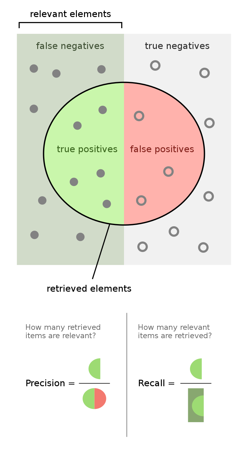
Recall

	Predicted Negative	Predicted Positive
Actually Negative	TN = 90 ✅	FP = 1 ❌
Actually Positive	FN = 8 ❌	TP = 1 ✅

Michigan Medicine test results

• 🤔 Question: What proportion of individuals who actually have COVID did the test identify?

• 🙋 Answer: $\frac{1}{1 + 8} = \frac{1}{9} \approx 0.11$.

• More generally, the recall of a binary classifier is the proportion of actually positive instances that are correctly classified. We'd like this number to be as close to 1 (100%) as possible.

$$\text{recall} = \frac{TP}{\text{# actually positive}} = \frac{TP}{TP + FN}$$

• To compute recall, look at the bottom (positive) row of the above confusion matrix.

Recall isn't everything, either!

$$\text{recall} = \frac{TP}{TP + FN}$$

• 🤔 Question: Can you design a "COVID test" with perfect recall?

• 🙋 Answer: Yes – just predict that everyone has COVID!

	Predicted Negative	Predicted Positive
Actually Negative	TN = 0 ✅	FP = 91 ❌
Actually Positive	FN = 0 ❌	TP = 9 ✅

everyone-has-COVID classifier

$$\text{recall} = \frac{TP}{TP + FN} = \frac{9}{9 + 0} = 1$$

• Like accuracy, recall on its own is not a perfect metric. Even though the classifier we just created has perfect recall, it has 91 false positives!

Precision

	Predicted Negative	Predicted Positive
Actually Negative	TN = 0 ✅	FP = 91 ❌
Actually Positive	FN = 0 ❌	TP = 9 ✅

everyone-has-COVID classifier

• The precision of a binary classifier is the proportion of predicted positive instances that are correctly classified. We'd like this number to be as close to 1 (100%) as possible.

$$\text{precision} = \frac{TP}{\text{# predicted positive}} = \frac{TP}{TP + FP}$$

• To compute precision, look at the right (positive) column of the above confusion matrix.
  Tip: A good way to remember the difference between precision and recall is that in the denominator for 🅿️recision, both terms have 🅿️ in them (TP and FP).

• Note that the "everyone-has-COVID" classifier has perfect recall, but a precision of $\frac{9}{9 + 91} = 0.09$, which is quite low.

• 🚨 Key idea: There is a "tradeoff" between precision and recall. Ideally, you want both to be high. For a particular prediction task, one may be important than the other.

• Later today, we'll see how to weigh this tradeoff in the context of selecting a threshold for classification in logistic regression.

Precision and recall

(source)

Discussion

$$\text{precision} = \frac{TP}{TP + FP} \: \: \: \: \: \: \: \: \text{recall} = \frac{TP}{TP + FN}$$

• 🤔 When might high precision be more important than high recall?

• 🤔 When might high recall be more important than high precision?

Activity

Consider the confusion matrix shown below.

	Predicted Negative	Predicted Positive
Actually Negative	TN = 22 ✅	FP = 2 ❌
Actually Positive	FN = 23 ❌	TP = 18 ✅

What is the accuracy of the above classifier? The precision? The recall?

After calculating all three on your own, click below to see the answers.

👉 Accuracy

(22 + 18) / (22 + 2 + 23 + 18) = 40 / 65

👉 Precision

18 / (18 + 2) = 9 / 10

👉 Recall

18 / (18 + 23) = 18 / 41

Activity

After fitting a BillyClassifier, we use it to make predictions on an unseen test set. Our results are summarized in the following confusion matrix.

	Predicted Negative	Predicted Positive
Actually Negative	???	30
Actually Positive	66	105

• Part 1: What is the recall of our classifier? Give your answer as a fraction (it does not need to be simplified).
  

• Part 2: The accuracy of our classifier is $\frac{69}{117}$. How many true negatives did our classifier have? Give your answer as an integer.
  

• Part 3: True or False: In order for a binary classifier's precision and recall to be equal, the number of mistakes it makes must be an even number.
  

• Part 4: Suppose we are building a classifier that listens to an audio source (say, from your phone’s microphone) and predicts whether or not it is Soulja Boy’s 2008 classic “Kiss Me thru the Phone." Our classifier is pretty good at detecting when the input stream is ”Kiss Me thru the Phone", but it often incorrectly predicts that similar sounding songs are also “Kiss Me thru the Phone."

Complete the sentence: Our classifier has...

• low precision and low recall.
• low precision and high recall.
• high precision and low recall.
• high precision and high recall.

Combining precision and recall

• If we care equally about a model's precision $PR$ and recall $RE$, we can combine the two using a single metric called the F1-score:

$$\text{F1-score} = \text{harmonic mean}(PR, RE) = 2\frac{PR \cdot RE}{PR + RE}$$

• Both F1-score and accuracy are overall measures of a binary classifier's performance. But remember, accuracy is misleading in the presence of class imbalance, and doesn't take into account the kinds of errors the classifier makes.

Other evaluation metrics for binary classifiers

• We just scratched the surface! This excellent table from Wikipedia summarizes the many other metrics that exist.

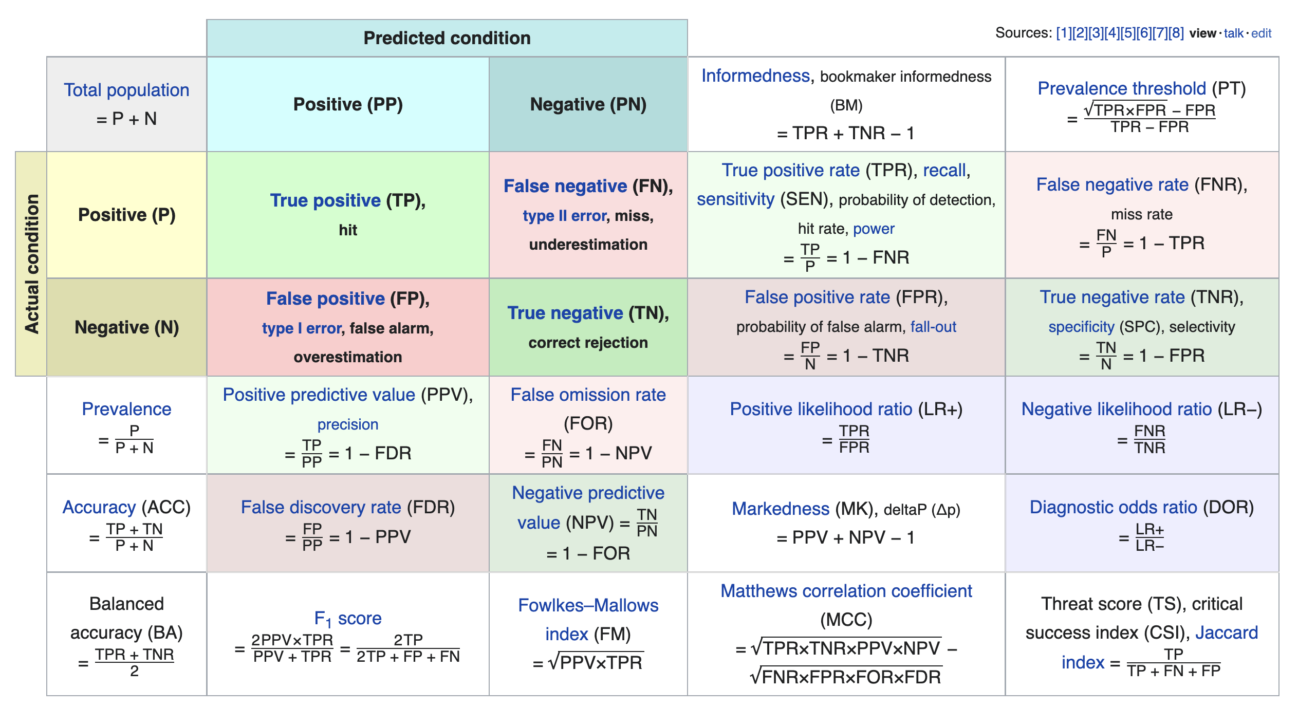
• If you're interested in exploring further, a good next metric to look at is true negative rate (i.e. specificity), which is the analogue of recall for true negatives.

Predicting probabilities

---

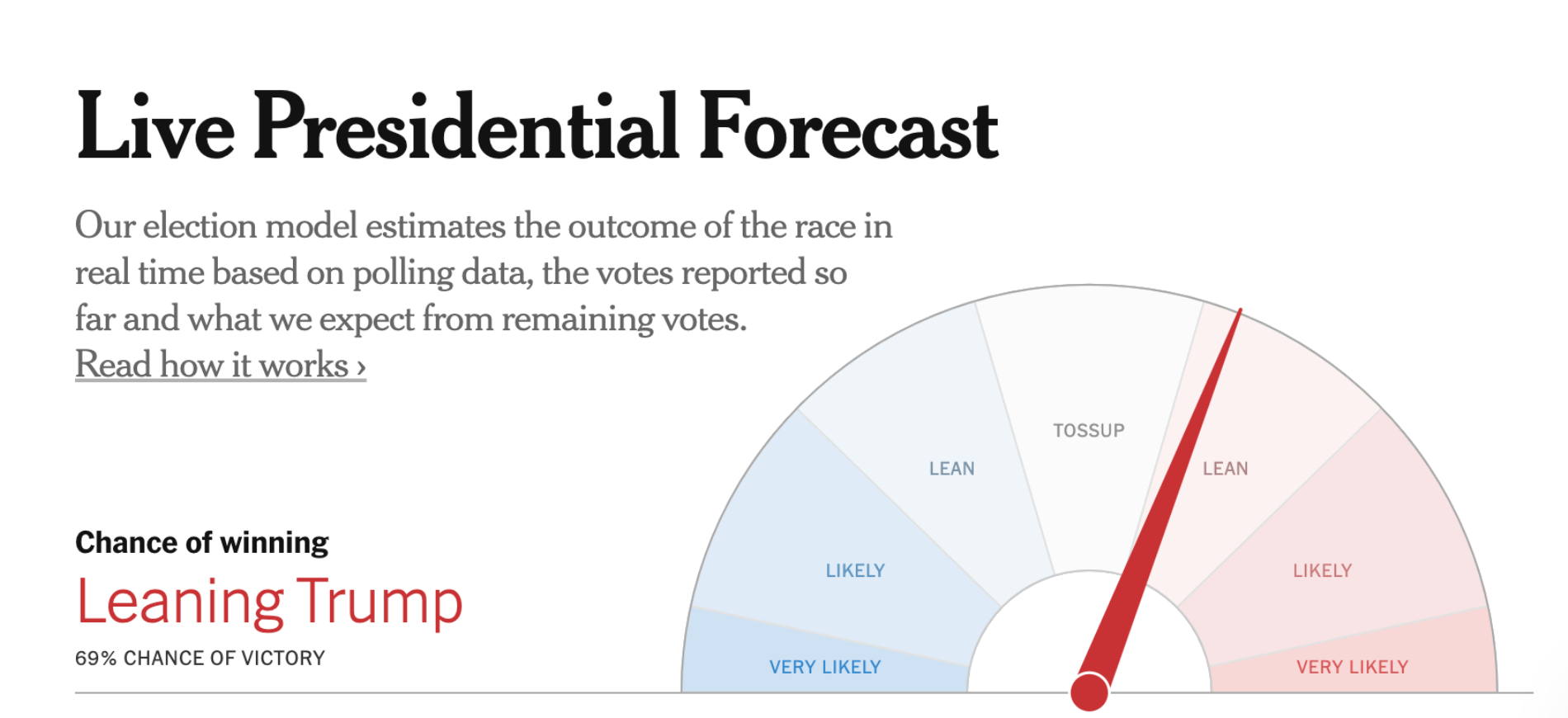
The New York Times maintained needles
that displayed the probabilities of various outcomes in the election.

Motivation: Predicting probabilities

• Often, we're interested in predicting the probability of an event occurring, given some other information.

Given that the score at the start of the second half is Michigan 23-Northwestern 15,
what's the probability that Michigan wins?

Here's a picture of an animal. What's the probability it's of a dog? Cat? Hamster? Zebra?

What's the probability that it snows on campus tomorrow?
In the context of weather apps, this is a nuanced question; here's a meme about it.

• If we're able to predict the probability of an event, we can classify the event by using a threshold.
  For example, if we predict there's a 70% chance of Michigan winning, we could predict that Michigan will win. Here, we implicitly used a threshold of 50%.

• The two classification techniques we've seen so far – $k$-Nearest Neighbors and decision trees – don't directly use probabilities in their decision-making process.
  But sometimes it's helpful to model uncertainty and to be able to state a level of confidence along with a prediction!

Recap: Predicting diabetes

• Let's try to predict whether or not a patient has diabetes ('Outcome') given just their 'Glucose' level.
  Last class, we used both 'Glucose' and 'BMI'; we'll start with just one feature for now.

• As before, class 0 (orange) is "no diabetes" and class 1 (blue) is "diabetes".

util.show_one_feature_plot(X_train, y_train)

• It seems that as a patient's 'Glucose' value increases, the chances they have diabetes also increases.

• Can we model this probability directly, as a function of 'Glucose'?
  In other words, can we find some $f$ such that:

$$P(y = 1 | \text{Glucose}) = f(\text{Glucose})$$

An attempt to predict probabilities

• Let's try and fit a simple linear model to the data from the previous slide.

util.show_one_feature_plot_with_linear_model(X_train, y_train)

• The simple linear model above predicts values greater than 1 and less than 0! This means we can't interpret the outputs as probabilities.

• We could, technically, clip the outputs of the linear model:

util.show_one_feature_plot_with_linear_model_clipped(X_train, y_train)

Bins and proportions

• Another approach we could try is to:
  • Place 'Glucose' values into bins, e.g. 50 to 55, 55 to 60, 60 to 65, etc.
  • Within each bin, compute the proportion of patients in the training set who had diabetes.

# Take a look at the source code in lec24_util.py to see how we did this!
# We've hidden a lot of the plotting code in the notebook to make it cleaner.
util.make_prop_plot(X_train, y_train)

• For example, the point near a 'Glucose' value of 100 has a $y$-axis value of ~0.25. This means that about 25% of patients with a 'Glucose' value near 100 had diabetes in the training set.

• So, if a new person comes along with a 'Glucose' value near 100, we'd predict there's a 25% chance they have diabetes (so they likely do not)!

• Notice that the points form an S-shaped curve!
  Can we incorporate this S-shaped curve in how we predict probabilities?

The logistic function

• The logistic function resembles an $S$-shape.

  $$\sigma(t) = \frac{1}{1 + e^{-t}} = \frac{1}{1 + \text{exp}(-t)}$$

  
  The logistic function is an example of a sigmoid function, which is the general term for an S-shaped function. Sometimes, we use the terms "logistic function" and "sigmoid function" interchangeably.

• Below, we'll look at the shape of $y = \sigma(w_0 + w_1 x)$ for different values of $w_0$ and $w_1$.
  • $w_0$ controls the position of the curve on the $x$-axis.
  • $w_1$ controls the "steepness" of the curve.

util.show_three_sigmoids()

• Notice that $0 < \sigma(t) < 1$, for all $t$, which means we can interpret the outputs of $\sigma(t)$ as probabilities!

• Below, interact with the sliders to change the values of $w_0$ and $w_1$.

interact(util.plot_sigmoid, w0=(-15, 15), w1=(-3, 3, 0.1));

interactive(children=(IntSlider(value=0, description='w0', max=15, min=-15), FloatSlider(value=0.0, descriptio…

Logistic regression

• Logistic regression is a linear classification technique that builds upon linear regression.

• It models the probability of belonging to class 1, given a feature vector:

$$P(y = 1 | \vec{x}) = \sigma (\underbrace{w_0 + w_1 x^{(1)} + w_2 x^{(2)} + ... + w_d x^{(d)}}_{\text{linear regression model}}) = \sigma\left(\vec{w} \cdot \text{Aug}(\vec{x}) \right)$$

• Note that the existence of coefficients, $w_0, w_1, ... w_d$, that we need to learn from the data, tells us that logistic regression is a parametric method!

LogisticRegression in sklearn

from sklearn.linear_model import LogisticRegression

• Let's fit a LogisticRegression classifier. Specifically, this means we're asking sklearn to learn the optimal parameters $w_0^*$ and $w_1^*$ in:

$$P(y = 1 | \text{Glucose}) = \sigma \left( w_0 + w_1 \cdot \text{Glucose} \right)$$

model_logistic = LogisticRegression()
model_logistic.fit(X_train[['Glucose']], y_train)

LogisticRegression()

In a Jupyter environment, please rerun this cell to show the HTML representation or trust the notebook.
On GitHub, the HTML representation is unable to render, please try loading this page with nbviewer.org.

• We get a test accuracy that's roughly in line with the test accuracies of the two models we saw last class.

model_logistic.score(X_test[['Glucose']], y_test)

0.7287234042553191

• What does our fit model look like?

Visualizing a fit logistic regression model

• The values of $w_0^*$ and $w_1^*$ sklearn found are below.

model_logistic.intercept_[0], model_logistic.coef_[0][0]

(-5.901585544378712, 0.04240496085762793)

• So, our fit model is:

$$P(y = 1 | \text{Glucose}) = \sigma(-5.9015855 + 0.04240496 \cdot \text{Glucose})$$

util.show_one_feature_plot_with_logistic(X_train, y_train)

• So, if a patient has a 'Glucose' level of 150, the model's predicted probability that they have diabetes is:

$$\sigma(-5.9015855 + 0.04240496 \cdot 150) \approx \sigma(0.46) \approx 0.61$$

model_logistic.predict_proba([[150]])

array([[0.39, 0.61]])

How did sklearn find $w_0^*$ and $w_1^*$?
What loss function did it use?

Cross-entropy loss

---

The modeling recipe

• To train a parametric model, we always follow the same three steps.

$k$-Nearest Neighbors and decision trees didn't quite follow the same process.

1. Choose a model.

$$P(y = 1 | \vec{x}) = \sigma (w_0 + w_1 x^{(1)} + w_2 x^{(2)} + ... + w_d x^{(d)}) = \sigma\left(\vec{w} \cdot \text{Aug}(\vec{x}) \right)$$

2. Choose a loss function.

???

3. Minimize average loss to find optimal model parameters.
   As we've now seen, average loss could also be regularized!

???

Attempting to use squared loss

• Our default loss function has always been squared loss, so we could try and use it here.

$$R_\text{sq}(\vec{w}) = \frac{1}{n} \sum_{i = 1}^n \left( y_i - \sigma\left(\vec{w} \cdot \text{Aug}(\vec{x}_i) \right) \right)^2$$

• Unfortunately, there's no closed form solution for $\vec{w}^*$, so we'll need to use gradient descent.

• Before doing so, let's visualize the loss surface in the case of our "simple" logistic model:

$$P(y = 1 | \text{Glucose}) = \sigma(w_0 + w_1 \cdot \text{Glucose})$$

• Specifically, we'll visualize:

$$R_\text{sq}(w_0, w_1) = \frac{1}{n} \sum_{i = 1}^n \left( y_i - \sigma(w_0 + w_1 \underbrace{x_i}_{\text{Glucose}_i} ) \right)^2$$

util.show_logistic_mse_surface(X_train, y_train)