from lec_utils import *
import lec23_util as util
from IPython.display import YouTubeVideo
from ipywidgets import interact
Announcements 📣
- The Portfolio Homework's checkpoint is due on Monday, November 25th – no slip days allowed!
The full homework is due on Saturday, December 7th (no slip days!). - Homework 10 will be out by tomorrow – sorry for the delay!
We'll adjust the deadline accordingly. - The Grade Report now includes scores and slip days through Homework 9 – make sure it's accurate!
Agenda
- Recap: Gradient descent for multivariate functions.
- Classification overview.
- Survey of classification methods.
- $k$-Nearest Neighbors 🏡🏠.
- Decision trees 🎄.
- Logistic regression 📈.
- Evaluating classifiers.
Question 🤔 (Answer at practicaldsc.org/q)
Remember that you can always ask questions anonymously at the link above!
Recap: Gradient descent for multivariate functions
Example: Gradient descent for simple linear regression
- To find optimal model parameters for the model $H(x) = w_0 + w_1 x$ and squared loss, we minimized empirical risk:
- This is a function of multiple variables, and is differentiable, so it has a gradient!
- Key idea: To find $\vec{w}^* = \begin{bmatrix} w_0^* \\ w_1^* \end{bmatrix}$, we could use gradient descent!
- Why would we, when closed-form solutions exist?
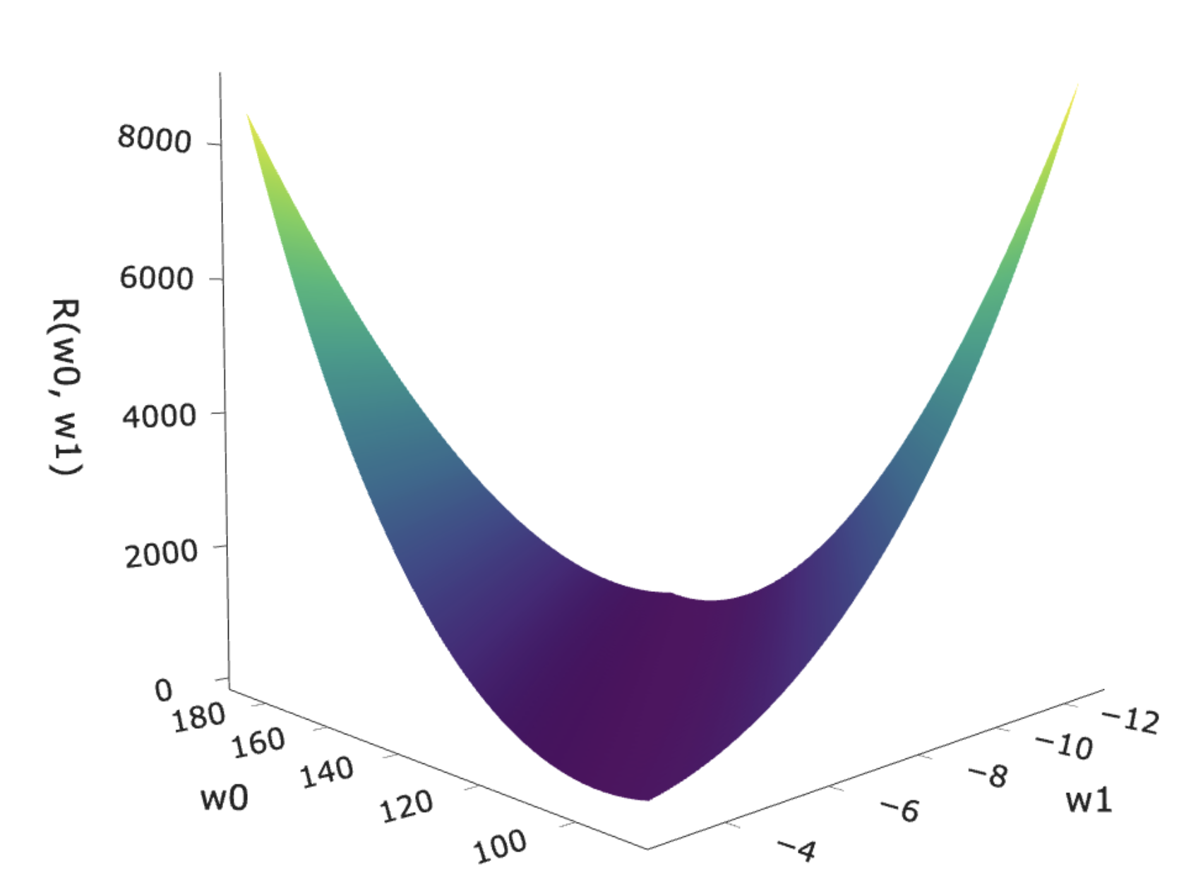
At any point, there are many directions in which you can go "up", but there's only one "steepest direction up", and that's the direction of the gradient!
Gradient descent for simple linear regression, visualized
YouTubeVideo('oMk6sP7hrbk')
Gradient descent for simple linear regression, implemented
- Let's use gradient descent to fit a simple linear regression model to predict commute time in
'minutes'from'departure_hour'.
df = pd.read_csv('data/commute-times.csv')
df[['departure_hour', 'minutes']]
util.make_scatter(df)
x = df['departure_hour']
y = df['minutes']
- First, let's remind ourselves what $w_0^*$ and $w_1^*$ are supposed to be.
slope = np.corrcoef(x, y)[0, 1] * np.std(y) / np.std(x)
slope
-8.186941724265557
intercept = np.mean(y) - slope * np.mean(x)
intercept
142.44824158772875
Implementing partial derivatives
def dR_w0(w0, w1):
return -2 * np.mean(y - (w0 + w1 * x))
def dR_w1(w0, w1):
return -2 * np.mean((y - (w0 + w1 * x)) * x)
Implementing gradient descent
- The update rule we'll follow is:
- We can treat this as two separate update equations:
- Let's initialize $w_0^{(0)} = 100$ and $w_1^{(0)} = -50$, and choose the step size $\alpha = 0.01$.
The initial guesses were just parameters that we thought might be close.
# We'll store our guesses so far, so we can look at them later.
def gradient_descent_for_regression(w0_initial, w1_initial, alpha, threshold=0.0001):
w0, w1 = w0_initial, w1_initial
w0_history = [w0]
w1_history = [w1]
while True:
w0 = w0 - alpha * dR_w0(w0, w1)
w1 = w1 - alpha * dR_w1(w0, w1)
w0_history.append(w0)
w1_history.append(w1)
if np.abs(w0_history[-1] - w0_history[-2]) <= threshold:
break
return w0_history, w1_history
w0_history, w1_history = gradient_descent_for_regression(0, 0, 0.01)
w0_history[-1]
142.1051891023626
w1_history[-1]
-8.146983792459055
- It seems that we converge at the right value! But how many iterations did it take? What could we do to speed it up?
len(w0_history)
20664
Classification overview
The taxonomy of machine learning
- So far, we've focused on building regression models.
- Regression is a form of supervised learning, in which the target variable (i.e., the $y$-values we're trying to predict) is numerical.
For example, a predicted commute time could technically be any real number.

- Next, we'll focus on classification, a form of supervised learning in which the target variable is categorical.
Example classification problems
- Does this person have diabetes?
This is an example of binary classification – there are only two possible classes, or categories. In binary classification, the two classes are typically 1 (yes) and 0 (no).
- Is this digit a 0, 1, 2, 3, 4, 5, 6, 7, 8, or 9?
This is an example of multi-class classification, where there are multiple possible classes.
- Will Michigan win this week?
- Is this picture of a dog, cat, zebra, or hamster?
The plan
- When we introduced regression, we started by understanding the theoretical foundations on paper, and then learned how to build models in
sklearn.
- This time, we'll do the reverse: we'll start by learning how to use classifiers in
sklearn, and then over the next few lectures, we'll dive deeper into the internals of a few.- $k$-Nearest Neighbors.
- Decision trees.
- Logistic regression.
Loading the data
- Our first classification example will involve predicting whether or not a patient has diabetes, given other information about their health.
diabetes = pd.read_csv('data/diabetes.csv')
display_df(diabetes, cols=9)
| Pregnancies | Glucose | BloodPressure | SkinThickness | Insulin | BMI | DiabetesPedigreeFunction | Age | Outcome | |
|---|---|---|---|---|---|---|---|---|---|
| 0 | 6 | 148 | 72 | 35 | 0 | 33.6 | 0.63 | 50 | 1 |
| 1 | 1 | 85 | 66 | 29 | 0 | 26.6 | 0.35 | 31 | 0 |
| 2 | 8 | 183 | 64 | 0 | 0 | 23.3 | 0.67 | 32 | 1 |
| ... | ... | ... | ... | ... | ... | ... | ... | ... | ... |
| 765 | 5 | 121 | 72 | 23 | 112 | 26.2 | 0.24 | 30 | 0 |
| 766 | 1 | 126 | 60 | 0 | 0 | 30.1 | 0.35 | 47 | 1 |
| 767 | 1 | 93 | 70 | 31 | 0 | 30.4 | 0.32 | 23 | 0 |
768 rows × 9 columns
# 0 means no diabetes, 1 means yes diabetes.
diabetes['Outcome'].value_counts()
Outcome 0 500 1 268 Name: count, dtype: int64
'Glucose'is measured in mg/dL (milligrams per deciliter).
'BMI'is calculated as $\text{BMI} = \frac{\text{weight (kg)}}{\left[ \text{height (m)} \right]^2}$.
- Let's start by using
'Glucose'and'BMI'to predict whether or not a patient has diabetes ('Outcome').
- But first, a train-test split:
from sklearn.model_selection import train_test_split
X_train, X_test, y_train, y_test = (
train_test_split(diabetes[['Glucose', 'BMI']], diabetes['Outcome'], random_state=1)
)
Visualizing the data
- Let's visualize the relationship between
X_trainandy_train. There are three numeric variables at play here –'Glucose','BMI', and'Outcome'– so we can use a 3D scatter plot.
px.scatter_3d(X_train.assign(Outcome=y_train),
x='Glucose', y='BMI', z='Outcome',
title='Relationship between Glucose, BMI, and Diabetes',
width=800, height=600)
- Since there are only two possible
'Outcome's, we can draw a 2D scatter plot of'BMI'vs.'Glucose'and color each point by'Outcome'. Below, class 0 (orange) is "no diabetes" and class 1 (blue) is "diabetes".
fig = (
X_train.assign(Outcome=y_train.astype(str).replace({'0': 'no diabetes', '1': 'yes diabetes'}))
.plot(kind='scatter', x='Glucose', y='BMI', color='Outcome',
color_discrete_map={'no diabetes': 'orange', 'yes diabetes': 'blue'},
title='Relationship between Glucose, BMI, and Diabetes')
.update_layout(width=800)
)
fig
- Using this dataset, how can we classify whether someone (not already in the dataset) has diabetes, given their
'Glucose'and'BMI'?
- Intuition: If a new person's feature vector is close to the blue points, we'll predict blue (diabetes); if they're close to the orange points, we'll predict orange (no diabetes).
Classifier 1: $k$-Nearest Neighbors 🏡🏠
$k$-Nearest Neighbors 🏡🏠
- Suppose we're given a new individual, $\vec{x}_\text{new} = \begin{bmatrix} \text{Glucose}_\text{new} \\ \text{BMI}_\text{new} \end{bmatrix}$.
- The $k$-Nearest Neighbors classifier ($k$-NN for short) classifies $\vec{x}_\text{new}$ by:
- Finding the $k$ closest points in the training set to $\vec{x}_\text{new}$.
- Predicting that $\vec{x}_\text{new}$ belongs to the most common class among those $k$ closest points.
fig
- Example: Suppose $k = 6$. If, among the 6 closest points to $\vec{x}_\text{new}$, there are 4 blue and 2 orange points, we'd predict blue (diabetes).
What if there are ties? Read here.
- $k$ is a hyperparameter that should be chosen through cross-validation.
As we've seen in Homework 9 (and 10!) in the context of $k$-NN regression, smaller values of $k$ tend to overfit significantly.
KNeighborsClassifier in sklearn
from sklearn.neighbors import KNeighborsClassifier
from sklearn.model_selection import GridSearchCV
- Let's fit a
KNeighborsClassifierby using cross-validation to choose a value of $k$ from 1 through 50.
Note thatKNeighborsClassifiers have several other hyperparameters. One of them is the metric used to measure distances; the default is the standard Euclidean (Pythagorean) distance, e.g. $\text{dist}(\vec u, \vec v) = \sqrt{(u_1 - v_1)^2 + (u_2 - v_2)^2 + ... + (u_d - v_d)^2}$.
model_knn = GridSearchCV(
KNeighborsClassifier(),
param_grid = {'n_neighbors': range(1, 51)}
)
model_knn.fit(X_train, y_train)
GridSearchCV(estimator=KNeighborsClassifier(),
param_grid={'n_neighbors': range(1, 51)})In a Jupyter environment, please rerun this cell to show the HTML representation or trust the notebook. On GitHub, the HTML representation is unable to render, please try loading this page with nbviewer.org.
GridSearchCV(estimator=KNeighborsClassifier(),
param_grid={'n_neighbors': range(1, 51)})KNeighborsClassifier(n_neighbors=28)
KNeighborsClassifier(n_neighbors=28)
model_knn.best_params_
{'n_neighbors': 28}
- Cross-validation chose $k = 28$. With the resulting model, we can make predictions using the
predictmethod, just like with regressors.
Note that all of the work in making the prediction – finding the 28 nearest neighbors, for instance – is done when we callpredict. "Training" does very little.
# To know what reasonable values for 'Glucose' and 'BMI' might be, let's look at the plot again.
fig
model_knn.predict(pd.DataFrame([{
'Glucose': 125,
'BMI': 40
}]))
array([0])
- What does the resulting model look like? Can we visualize it?
Decision boundaries
- The decision boundaries of a classifier visualize the regions in the feature space that separate different predicted classes.
- The decision boundaries for
model_knnare visualized below.
If a new person's feature vector lies in the blue region, we'd predict they do have diabetes, otherwise, we'd predict they don't.
util.show_decision_boundary(model_knn, X_train, y_train, title='Decision Boundary when $k = 28$')

- What would the decision boundaries look like if $k$ increased or decreased?
Play with the slider below to find out!
from ipywidgets import interact
interact(lambda k: util.visualize_k(k, X_train, y_train), k=(1, 51));
interactive(children=(IntSlider(value=26, description='k', max=51, min=1), Output()), _dom_classes=('widget-in…
- What if $k = n$, the number of points in the training set?
util.visualize_k(576, X_train, y_train)

Quantifying the performance of a classifier
- For regression models, our default evaluation metric was mean squared error.
Error is bad, so lower values indicate better model performance.
The most common evaluation metric in classification is accuracy:
$$\text{accuracy} = \frac{\text{# data points classified correctly}}{\text{# data points}}$$
Accuracy ranges from 0 to 1, i.e. 0% to 100%. Higher values indicate better model performance.
# Equivalent to 75%.
(model_knn.predict(X_test) == y_test).mean()
0.75
- This is the default metric that the
scoremethod of a classifier computes, too.
model_knn.score(X_test, y_test)
0.75
# For future reference.
test_scores = pd.Series()
test_scores['knn with k = 28'] = model_knn.score(X_test, y_test)
test_scores
knn with k = 28 0.75 dtype: float64
- Accuracy is not the only metric we care about, and can sometimes be misleading. More on this soon!
Activity
It seems that a $k$-NN classifier that uses $k = 1$ should achieve 100% training accuracy. Why doesn't the model defined below have 100% training accuracy?
model_k1 = KNeighborsClassifier(n_neighbors=1)
model_k1.fit(X_train, y_train)
KNeighborsClassifier(n_neighbors=1)In a Jupyter environment, please rerun this cell to show the HTML representation or trust the notebook.
On GitHub, the HTML representation is unable to render, please try loading this page with nbviewer.org.
KNeighborsClassifier(n_neighbors=1)
# Training accuracy – high, but not 100%.
model_k1.score(X_train, y_train)
0.9913194444444444
# Accuracy on test set is lower than when k = 28!
model_k1.score(X_test, y_test)
0.6822916666666666
test_scores['knn with k = 1'] = model_k1.score(X_test, y_test)
test_scores
knn with k = 28 0.75 knn with k = 1 0.68 dtype: float64
Discussion
Why should we generally standardize features before using a $k$-NN classifier?
X_train_scaled = X_train.copy()
X_train_scaled['Glucose * 2'] = X_train_scaled['Glucose'] * 2
(
X_train_scaled.assign(Outcome=y_train.astype(str).replace({'0': 'no diabetes', '1': 'yes diabetes'}))
.plot(kind='scatter', x='Glucose * 2', y='BMI', color='Outcome',
color_discrete_map={'no diabetes': 'orange', 'yes diabetes': 'blue'},
title='Relationship between Glucose * 2, BMI, and Diabetes')
.update_layout(width=1300)
.update_xaxes(tickvals=np.arange(0, 500, 100))
)
fig
Parametric vs. non-parametric models
- The $k$-Nearest Neighbors classifier is an example of a non-parametric machine learning method.
- Linear regression, on the other hand, is parametric.
- Some differences between parametric and non-parametric models:
| Parametric | Non-Parametric |
|---|---|
| There's a fixed set of coefficients (parameters), $w_0, w_1, ..., w_d$ that we'll use for making predictions, and the number of coefficients is independent of the training set size. | No fixed set of parameters; model complexity increases as the training set size increases. |
| Parametric methods make assumptions about the shape of the data and/or its underlying probability distribution. For instance, linear models assume a linear relationship between the features $X$ and target $\vec{y}$. There's a connection between the squared loss function and maximum likelihood estimation, too. |
Non-parametric methods make no assumptions about the shape of the data. |
Classifier 2: Decision trees 🎄
Decision trees 🎄
- Suppose we're given a new individual, $\vec{x}_\text{new} = \begin{bmatrix} \text{Glucose}_\text{new} \\ \text{BMI}_\text{new} \end{bmatrix}$.
- The decision tree classifier classifies $\vec{x}_\text{new}$ by:
- Asking a series of yes/no questions about $\text{Glucose}_\text{new}$ and $\text{BMI}_\text{new}$, e.g.:
Is $\text{Glucose}_\text{new} \leq 129.5$? 2. Once it runs out of questions to ask, it predicts that $\vec{x}_\text{new}$ belongs to the **most common class** among training set points that had the same answers as $\vec{x}_\text{new}$.
If so, is $\text{BMI}_\text{new} \leq 26.3$?
If not, is $\text{BMI}_\text{new} \leq 29.95$?
$\vdots$
- Visually, a fit decision tree may look like:
- Decision trees are also non-parametric!
DecisionTreeClassifier in sklearn
from sklearn.tree import DecisionTreeClassifier
- Let's fit a
DecisionTreeClassifier.
One of the main hyperparameters ismax_depth, the number of questions to ask before making a prediction. Typically, we fit this with cross-validation, but for now we'll hard-code it.
model_tree = DecisionTreeClassifier(max_depth=3)
model_tree.fit(X_train, y_train)
DecisionTreeClassifier(max_depth=3)In a Jupyter environment, please rerun this cell to show the HTML representation or trust the notebook.
On GitHub, the HTML representation is unable to render, please try loading this page with nbviewer.org.
DecisionTreeClassifier(max_depth=3)
- The decision tree achieves a slightly higher test set accuracy than the cross-validated $k$-NN model.
model_tree.score(X_test, y_test)
0.7708333333333334
test_scores['decision tree with depth = 3'] = model_tree.score(X_test, y_test)
test_scores
knn with k = 28 0.75 knn with k = 1 0.68 decision tree with depth = 3 0.77 dtype: float64
- But what does it look like?
Decision boundaries for a decision tree classifier
util.show_decision_boundary(model_tree, X_train, y_train, title='Decision Boundary for a Tree of Depth 3')

- Observe that the decision boundaries – at least when we set
max_depthto 3 – look less "jagged" than with the $k$-NN classifier.
Visualizing decision trees
- Our fit decision tree is like a "flowchart", made up of a series of questions.
It turns outsklearnprovides us with a convenient way of visualizing this flowchart.
- As before, orange is "no diabetes" and blue is "diabetes".
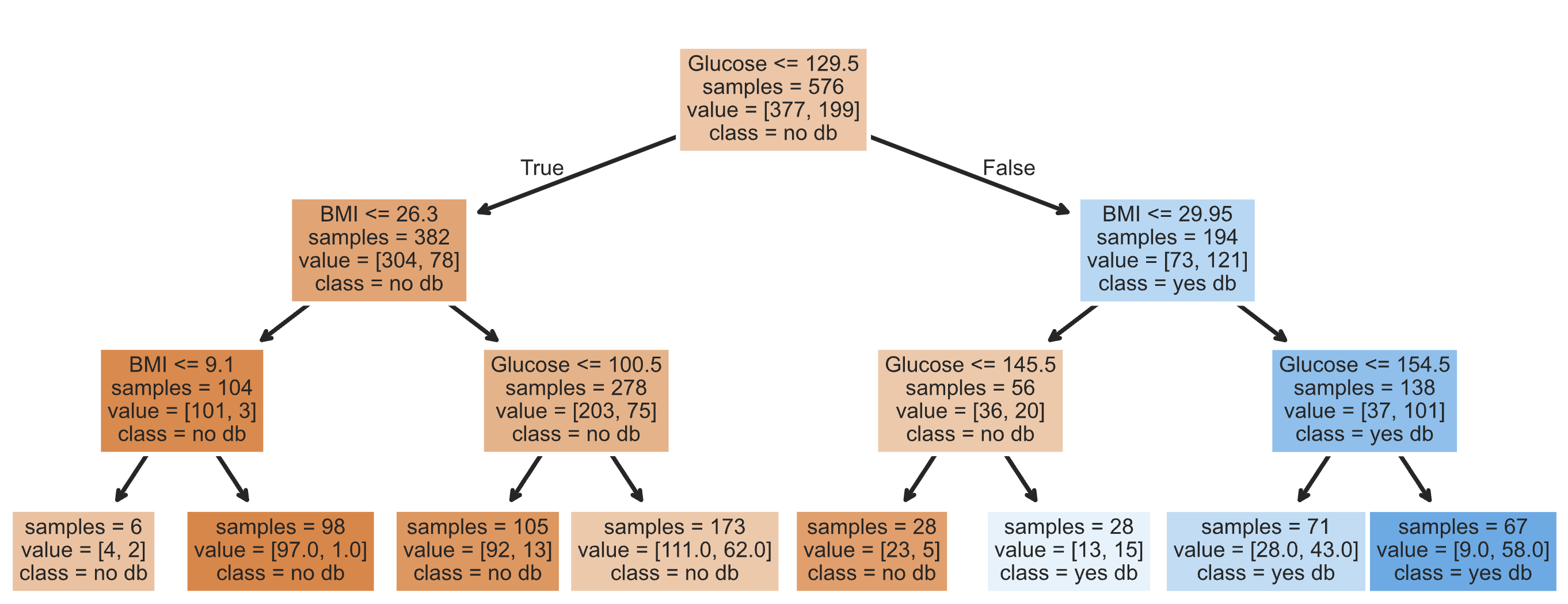
from sklearn.tree import plot_tree
plt.figure(figsize=(13, 5))
plot_tree(model_tree, feature_names=X_train.columns, class_names=['no db', 'yes db'],
filled=True, fontsize=10, impurity=False);

- To classify a new data point, we start at the top and answer the first question (i.e. "Glucose <= 129.5").
- If the answer is "Yes", we move to the left branch, otherwise we move to the right branch.
- We repeat this process until we end up at a leaf node, at which point we predict the most common class in that node.
Note that each node has avalueattribute, which describes the number of training individuals of each class that fell in that node.
y_train[X_train[X_train['Glucose'] <= 129.5].index].value_counts()
Outcome 0 304 1 78 Name: count, dtype: int64
Increasing tree depth
- One of the many hyperparameters we can tune is tree depth.
- What happens to the decision boundary of the resulting classifier if we increase
max_depth?
interact(lambda depth: util.visualize_depth(depth, X_train, y_train), depth=(1, 51));
interactive(children=(IntSlider(value=26, description='depth', max=51, min=1), Output()), _dom_classes=('widge…
- What happens to the flowchart representation of the resulting classifier if we increase
max_depth?
# By default, there is pre-specified maximum depth.
# The training algorithm keeps
model_tree_no_max = DecisionTreeClassifier()
model_tree_no_max.fit(X_train, y_train)
DecisionTreeClassifier()In a Jupyter environment, please rerun this cell to show the HTML representation or trust the notebook.
On GitHub, the HTML representation is unable to render, please try loading this page with nbviewer.org.
DecisionTreeClassifier()
# Uncomment this!
# plt.figure(figsize=(5, 5))
# plot_tree(model_tree_no_max, feature_names=X_train.columns, class_names=['no db', 'yes db'],
# filled=True, fontsize=10, impurity=False);
- The tree is extremely overfit to the training set, and very deep!
# Training accuracy. This number should look familiar!
model_tree_no_max.score(X_train, y_train)
0.9913194444444444
model_tree_no_max.tree_.max_depth
21
# Worse test set performance than when we used max_depth = 3!
test_scores['decision tree with no specified max depth'] = model_tree_no_max.score(X_test, y_test)
test_scores
knn with k = 28 0.75 knn with k = 1 0.68 decision tree with depth = 3 0.77 decision tree with no specified max depth 0.71 dtype: float64
Lingering questions about decision trees
- How are decision trees fit – that is, how do they decide what questions to ask?
- Other than limiting the depth of a decision tree, how else can we scale back the complexity of a decision tree (to hopefully help with model generalizability)? What is a random forest?
- Can they be used for regression, too?
- We'll address these ideas next week.

Classifier 3: Logistic regression 📈
Logistic regression 📈
- Logistic regression is a linear classification technique that builds upon linear regression.
- It models the probability of belonging to class 1, given a feature vector:
- Here, $\sigma(t) = \frac{1}{1 + e^{-t}}$ is the sigmoid function; its outputs are between 0 and 1, which means they can be interpreted as probabilities.
The predictions of a "regular" linear regression model can be anything from $-\infty$ to $+\infty$, meaning they can't be interpreted as probabilities.
- Note that the existence of coefficients, $w_0, w_1, ... w_d$, that we need to learn from the data, tells us that logistic regression is a parametric method!
Predicting probabilities vs. predicting classes
- 🤔 Question: Suppose our logistic regression model predicts the probability that someone has diabetes is 0.75. What do we predict – diabetes or no diabetes? What if the predicted probability is 0.3?
- 🙋 Answer: We have to pick a threshold (for example, 0.5)!
- If the predicted probability is above the threshold, we predict diabetes (1).
- Otherwise, we predict no diabetes (0).
The sigmoid function
- The sigmoid function, also known as the logistic function, resembles an $S$-shape.
- Below, we'll look at the shape of $y = \sigma(w_0 + w_1 x)$ for different values of $w_0$ and $w_1$.
- $w_0$ controls the position of the curve on the $x$-axis.
- $w_1$ controls the "steepness" of the curve.
# If this doesn't render in the HTML, see the notebook on GitHub or the recording!
util.show_three_sigmoids()
- Below, interact with the sliders to change the values of $w_0$ and $w_1$.
# If this doesn't render in the HTML, see the notebook on GitHub or the recording!
interact(util.plot_sigmoid, w0=(-15, 15), w1=(-15, 15));
interactive(children=(IntSlider(value=0, description='w0', max=15, min=-15), IntSlider(value=0, description='w…
LogisticRegression in sklearn
from sklearn.linear_model import LogisticRegression
- Let's fit a
LogisticRegressionclassifier. Specifically, this means we're askingsklearnto learn the optimal parameters $w_0^*$, $w_1^*$, and $w_2^*$ in:
- The most common loss function for logistic regression isn't squared loss, rather it's cross-entropy loss (also known as log loss); more on this next class.
- By default,
sklearnuses $L_2$ regularization for logistic regression. It doesn't cross-validate for $\lambda$ unless we tell it to; by default, it uses $\lambda = 1$.
model_logistic = LogisticRegression()
model_logistic.fit(X_train, y_train)
LogisticRegression()In a Jupyter environment, please rerun this cell to show the HTML representation or trust the notebook.
On GitHub, the HTML representation is unable to render, please try loading this page with nbviewer.org.
LogisticRegression()
- The test accuracy, without any cross-validation for the regularization hyperparameter, is about the same as the other not-super-overfit models.
model_logistic.score(X_test, y_test)
0.765625
test_scores['logistic regression'] = model_logistic.score(X_test, y_test)
test_scores.to_frame()
| 0 | |
|---|---|
| knn with k = 28 | 0.75 |
| knn with k = 1 | 0.68 |
| decision tree with depth = 3 | 0.77 |
| decision tree with no specified max depth | 0.71 |
| logistic regression | 0.77 |
- But again, we should ask, what does it look like?
Predicting probabilities vs. predicting classes, revisited
- By default, the
predictmethod of a fitLogisticRegressionmodel predicts a class.
model_logistic.predict(pd.DataFrame([{
'Glucose': 125,
'BMI': 40
}]))
array([0])
- But, logistic regression is designed to predict probabilities. We can access these predicted probabilities using the
predict_probamethod.
model_logistic.predict_proba(pd.DataFrame([{
'Glucose': 125,
'BMI': 40
}]))
array([[0.52, 0.48]])
- The above is telling us that the model thinks this person has:
- A 52% chance of belonging to class 0 (no diabetes).
- A 48% chance of belonging to class 1 (diabetes).
- By default, it uses a threshold of 0.5, i.e. it predicts the larger probability. As we'll soon discuss, this may not be what we want!
Unfortunately,sklearndoesn't let us change the threshold ourselves. If we want a different threshold, we need to manually implement it using the results ofpredict_proba.
Decision boundaries for logistic regression
util.show_decision_boundary(model_logistic, X_train, y_train, title='Decision Boundary for Logistic Regression')

- Unlike other models, this decision boundary is linear! Next class, we'll see how to find the equation of the line that separates the two classes, and how it relates to the coefficients and intercept below.
model_logistic.intercept_, model_logistic.coef_
(array([-7.62]), array([[0.04, 0.08]]))
- But where does the sigmoid curve $\sigma(t)$ appear, in the context of making predictions?
Visualizing the probability of belonging to class 1
- Recall, the logistic regression model is trained to predict the probability of class 1 (diabetes).
- The graph below shows the predicted probabilities of class 1 (diabetes) for different combinations of features.
util.show_logistic(model_logistic, X_train, y_train)
- Play with the slider below to change the threshold that's used to classify an individual as class 1 (diabetes) or class 0 (no diabetes)!
interact(lambda t: util.show_logistic(model_logistic, X_train, y_train, show_threshold=True, t=t), t=(0, 1, 0.05));
interactive(children=(FloatSlider(value=0.0, description='t', max=1.0, step=0.05), Output()), _dom_classes=('w…
- The introduction of the threshold creates a decision boundary, which is reflected in the 2D plot we saw a few slides ago.
util.show_decision_boundary(model_logistic, X_train, y_train, title='Decision Boundary for Logistic Regression')

Lingering questions about logistic regression
- What loss function do we use to find optimal model parameters for logistic regression?
- How do we interpret the resulting coefficients?
- What assumptions does the logistic regression model make?
The linear regression model assumes the output is a linear combination of features. Part of the logistic regression model resembles the linear regression model, so presumably, something in logistic regression is a linear combination of features, but what?
- We'll address these ideas next class.
Classifier evaluation
Accuracy isn't everything!
$$ \text{accuracy} = \frac{\text{# data points classified correctly}}{\text{# data points}} $$- Accuracy is defined as the proportion of predictions that are correct.
- It weighs all correct predictions the same, and weighs all incorrect predictions the same.
- But some incorrect predictions may be worse than others!
- Suppose you take a COVID test 🦠. Which is worse:
- The test saying you have COVID, when you really don't, or
- The test saying you don't have COVID, when you really do?
- Suppose you take a COVID test 🦠. Which is worse:
Outcomes in binary classification
- When performing binary classification, there are four possible outcomes.
Note: A "positive prediction" is a prediction of 1, and a "negative prediction" is a prediction of 0.
| Outcome of Prediction | Definition | True Class |
|---|---|---|
| True positive (TP) ✅ | The predictor correctly predicts the positive class. | P |
| False negative (FN) ❌ | The predictor incorrectly predicts the negative class. | P |
| True negative (TN) ✅ | The predictor correctly predicts the negative class. | N |
| False positive (FP) ❌ | The predictor incorrectly predicts the positive class. | N |
- We typically organize the four quantities above into a confusion matrix.
| Predicted Negative | Predicted Positive | |
|---|---|---|
| Actually Negative | TN ✅ | FP ❌ |
| Actually Positive | FN ❌ | TP ✅ |
- Note that in the four acronyms – TP, FN, TN, FP – the first letter is whether the prediction is correct, and the second letter is what the prediction is.
Example: COVID testing 🦠
- Michigan Medicine administers hundreds of COVID tests a day. The tests are not fully accurate.
- Each test comes back either:
- positive, indicating that the individual has COVID, or
- negative, indicating that the individual does not have COVID.
- Question: What is a TP in this scenario? FP? TN? FN?
- TP: The test predicted that the individual has COVID, and they do ✅.
- FP: The test predicted that the individual has COVID, but they don't ❌.
- TN: The test predicted that the individual doesn't have COVID, and they don't ✅.
- FN: The test predicted that the individual doesn't have COVID, but they do ❌.
Accuracy of COVID tests
- The results of 100 Michigan Medicine COVID tests are given below.
| Predicted Negative | Predicted Positive | |
|---|---|---|
| Actually Negative | TN = 90 ✅ | FP = 1 ❌ |
| Actually Positive | FN = 8 ❌ | TP = 1 ✅ |
- 🤔 Question: What is the accuracy of the test?
- 🙋 Answer: $$\text{accuracy} = \frac{TP + TN}{TP + FP + FN + TN} = \frac{1 + 90}{100} = 0.91$$
- Followup: At first, the test seems good. But, suppose we build a classifier that predicts that nobody has COVID. What would its accuracy be?
- Answer to followup: Also 0.91! There is severe class imbalance in the dataset, meaning that most of the data points are in the same class (no COVID). Accuracy doesn't tell the full story.
Recall
| Predicted Negative | Predicted Positive | |
|---|---|---|
| Actually Negative | TN = 90 ✅ | FP = 1 ❌ |
| Actually Positive | FN = 8 ❌ | TP = 1 ✅ |
- 🤔 Question: What proportion of individuals who actually have COVID did the test identify?
- 🙋 Answer: $\frac{1}{1 + 8} = \frac{1}{9} \approx 0.11$.
- More generally, the recall of a binary classifier is the proportion of actually positive instances that are correctly classified. We'd like this number to be as close to 1 (100%) as possible.
- To compute recall, look at the bottom (positive) row of the above confusion matrix.
Recall isn't everything, either!
$$\text{recall} = \frac{TP}{TP + FN}$$- 🤔 Question: Can you design a "COVID test" with perfect recall?
- 🙋 Answer: Yes – just predict that everyone has COVID!
| Predicted Negative | Predicted Positive | |
|---|---|---|
| Actually Negative | TN = 0 ✅ | FP = 91 ❌ |
| Actually Positive | FN = 0 ❌ | TP = 9 ✅ |
- Like accuracy, recall on its own is not a perfect metric. Even though the classifier we just created has perfect recall, it has 91 false positives!
Precision
| Predicted Negative | Predicted Positive | |
|---|---|---|
| Actually Negative | TN = 0 ✅ | FP = 91 ❌ |
| Actually Positive | FN = 0 ❌ | TP = 9 ✅ |
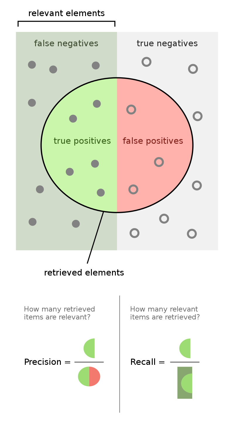
- The precision of a binary classifier is the proportion of predicted positive instances that are correctly classified. We'd like this number to be as close to 1 (100%) as possible.
- To compute precision, look at the right (positive) column of the above confusion matrix.
Tip: A good way to remember the difference between precision and recall is that in the denominator for 🅿️recision, both terms have 🅿️ in them (TP and FP).
- Note that the "everyone-has-COVID" classifier has perfect recall, but a precision of $\frac{9}{9 + 91} = 0.09$, which is quite low.
- 🚨 Key idea: There is a "tradeoff" between precision and recall. Ideally, you want both to be high. For a particular prediction task, one may be important than the other.
- Next class, we'll see how to weigh this tradeoff in the context of selecting a threshold for classification in logistic regression.
Discussion
$$\text{precision} = \frac{TP}{TP + FP} \: \: \: \: \: \: \: \: \text{recall} = \frac{TP}{TP + FN}$$🤔 When might high precision be more important than high recall?
🤔 When might high recall be more important than high precision?
Activity
Consider the confusion matrix shown below.
| Predicted Negative | Predicted Positive | |
|---|---|---|
| Actually Negative | TN = 22 ✅ | FP = 2 ❌ |
| Actually Positive | FN = 23 ❌ | TP = 18 ✅ |
What is the accuracy of the above classifier? The precision? The recall?
After calculating all three on your own, click below to see the answers.
👉 Accuracy
(22 + 18) / (22 + 2 + 23 + 18) = 40 / 65👉 Precision
18 / (18 + 2) = 9 / 10👉 Recall
18 / (18 + 23) = 18 / 41Activity
After fitting a BillyClassifier, we use it to make predictions on an unseen test set. Our results are summarized in the following confusion matrix.
| Predicted Negative | Predicted Positive | |
|---|---|---|
| Actually Negative | ??? | 30 |
| Actually Positive | 66 | 105 |
Part 1: What is the recall of our classifier? Give your answer as a fraction (it does not need to be simplified).
Part 2: The accuracy of our classifier is $\frac{69}{117}$. How many true negatives did our classifier have? Give your answer as an integer.
Part 3: True or False: In order for a binary classifier's precision and recall to be equal, the number of mistakes it makes must be an even number.
Part 4: Suppose we are building a classifier that listens to an audio source (say, from your phone’s microphone) and predicts whether or not it is Soulja Boy’s 2008 classic “Kiss Me thru the Phone." Our classifier is pretty good at detecting when the input stream is ”Kiss Me thru the Phone", but it often incorrectly predicts that similar sounding songs are also “Kiss Me thru the Phone."
Complete the sentence: Our classifier has...
- low precision and low recall.
- low precision and high recall.
- high precision and low recall.
- high precision and high recall.
Combining precision and recall
- If we care equally about a model's precision $PR$ and recall $RE$, we can combine the two using a single metric called the F1-score:
- Both F1-score and accuracy are overall measures of a binary classifier's performance. But remember, accuracy is misleading in the presence of class imbalance, and doesn't take into account the kinds of errors the classifier makes.
Other evaluation metrics for binary classifiers
- We just scratched the surface! This excellent table from Wikipedia summarizes the many other metrics that exist.
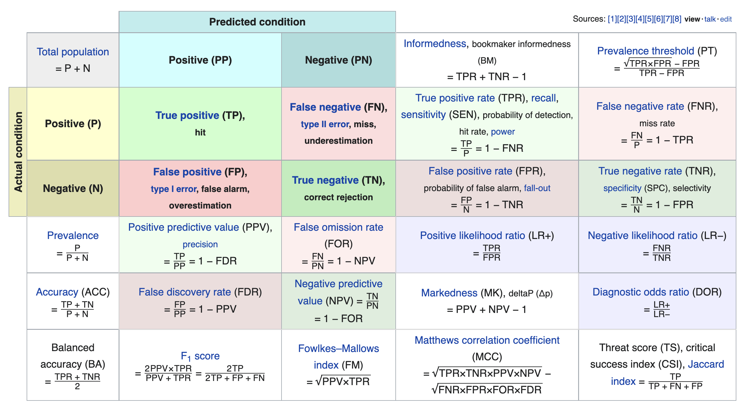
- If you're interested in exploring further, a good next metric to look at is true negative rate (i.e. specificity), which is the analogue of recall for true negatives.