from lec_utils import *
import lec20_util as util
def show_cv_slides():
    src = "https://docs.google.com/presentation/d/e/2PACX-1vTydTrLDr-y4nxQu1OMsaoqO5EnPEISz2VYmM6pd83ke8YnnTBJlp40NfNLI1HMgoaKx6GBKXYE4UcA/embed?start=false&loop=false&delayms=60000&rm=minimal"
    display(IFrame(src, width=900, height=361))
import warnings
warnings.simplefilter('ignore')
Announcements 📣
- Homework 9 is due on Monday, November 11th.
We're adding more office hours tomorrow and on Monday. - The Portfolio Homework has been released! Read all about it here. It has two due dates:
- A checkpoint (worth 15 points / 100) is due on Monday, November 25th (no slip days!).
- The full homework is due on Saturday, December 7th (no slip days!).
- Homework 8 solutions can be found in #282 on Ed, and Homework 7 solutions can be found in #259 on Ed.
- Please help spread the word about this class by submitting an anonymous testimony here 🙏.
We'll share some of the responses we get on this form at practicaldsc.org/next, and in advertisement emails/posts we share with other students.

Agenda
- Recap: Generalization, hyperparameters, and train-test splits.
- Cross-validation.
- Grid search.
- Regularization.
Additional resources
- Take a look at mlu-explain.github.io, a site with interactive explanations for a lot of core machine learning topics, like:
- Linear Regression.
- The Bias-Variance Tradeoff.
- Train, Test, and Validation Sets.
- Cross-Validation.
- and other ideas we'll see later in the semester!
- We've linked these articles in the Resources tab of the course website, too.
Question 🤔 (Answer at practicaldsc.org/q)
Remember that you can always ask questions anonymously at the link above!
Recap: Generalization, hyperparameters, and train-test splits
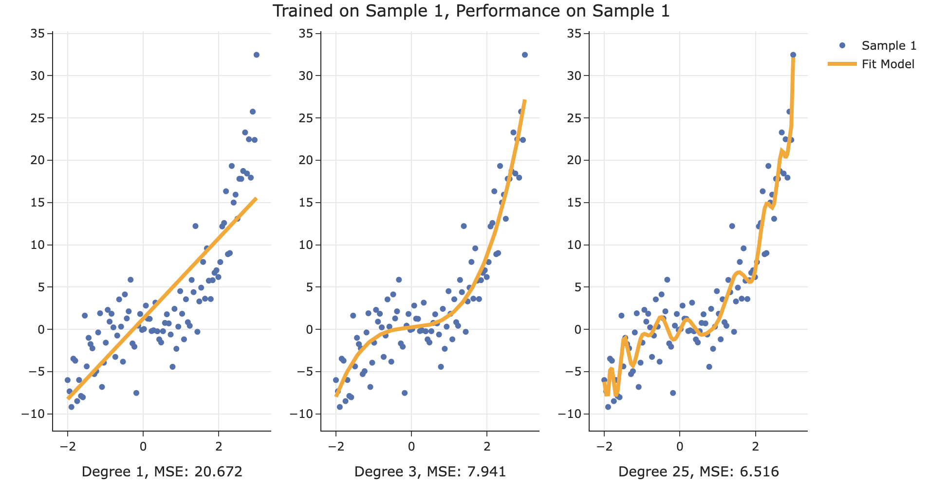
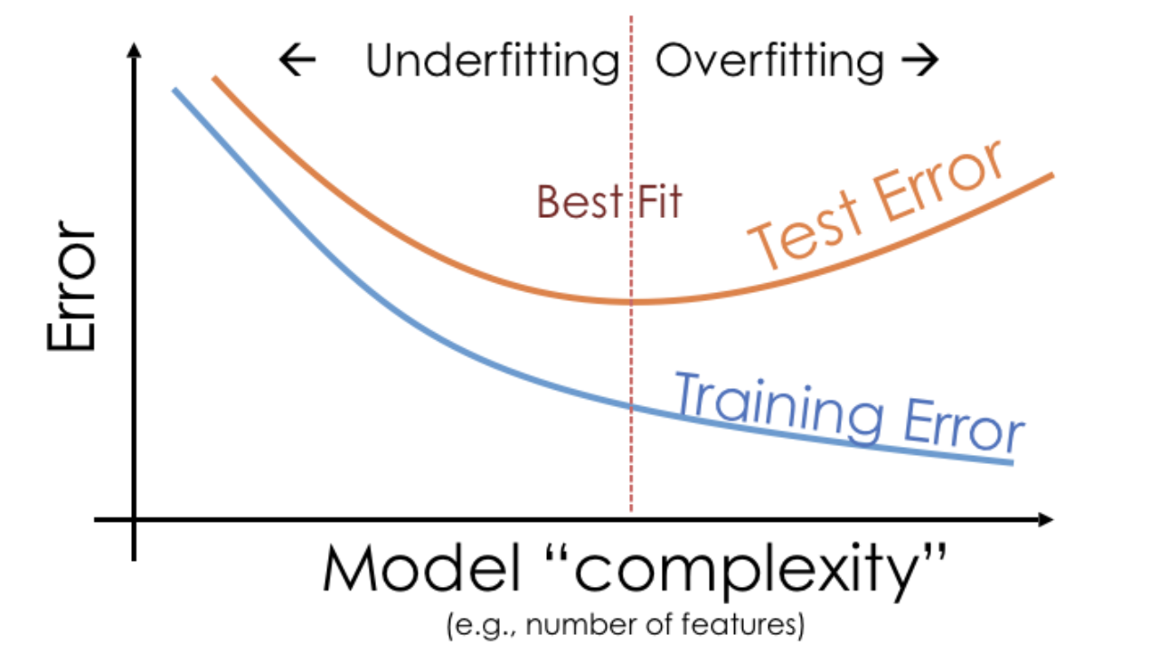
As we increase the complexity (e.g., polynomial degree) of our models, their training error decreases.
Here, polynomial degree is a hyperparameter – something we get to choose before fitting the model to the data. We're trying to determine how to choose the "best" hyperparameter.
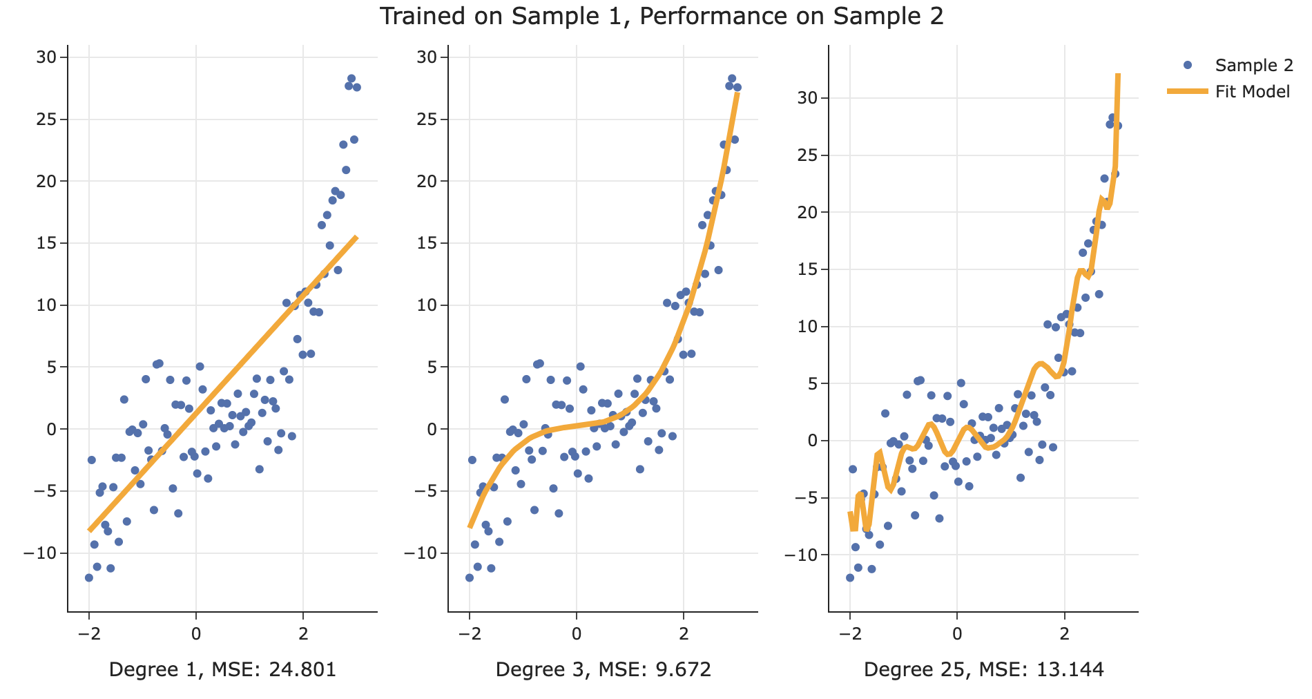
But, as we increase complexity, our models overfit to their training data, and can fail to generalize to unseen, test data.
Generalization
- We care about how well our models generalize to unseen data.
- The more complex a model is, the more it will overfit to the noise in the training data, and have high model variance.
- The less complex a model is, the more it will underfit the training data, and have high bias.
- To navigate this bias-variance tradeoff, we choose model complexity by choosing the model with the lowest error on an unseen test set.
Conducting train-test splits
- Recall, training data is used to fit our model, and test data is used to evaluate our model.
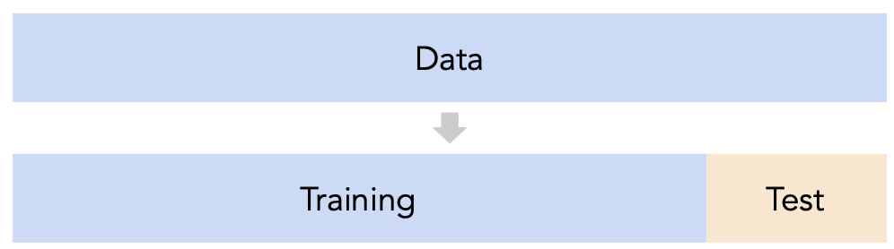
- Question: How should we split?
sklearn'strain_test_splitsplits randomly, which usually works well.- However, if there is some element of time in the training data (say, when predicting the future price of a stock), a better split is "past" and "future".
- Question: How large should the split be, e.g. 90%-10% vs. 75%-25%?
- There's a tradeoff – a larger training set should lead to a "better" model, while a larger test set should lead to a better estimate of our model's ability to generalize.
- There's no "right" choice, but we usually choose between 10% to 25% for the test set.
But wait...
- With our current strategy, we are choosing the hyperparameter that creates the model that performs best on the test set.
- As such, we are overfitting to the test set – the best hyperparameter for the test set might not be the best hyperparameter for a totally unseen dataset!
- It seems like we need another split.
- Next, we'll cover the more robust solution to the problem of selecting hyperparameters: cross-validation.
Cross-validation
Idea: A single validation set
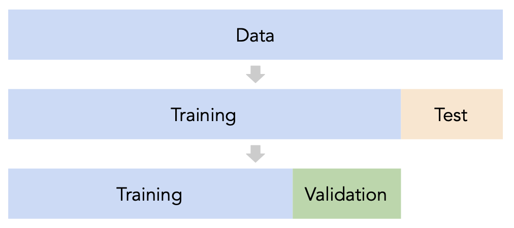
- Split the data into three sets: training, validation, and test.
- For each hyperparameter choice, train the model only on the training set, and evaluate the model's performance on the validation set.
- Find the hyperparameter with the best validation performance.
- Retrain the final model on the training and validation sets, and report its performance on the test set.
- Issue: This strategy is too dependent on the validation set, which may be small and/or not a representative sample of the data. We're not going to do this. ❌
A better idea: $k$-fold cross-validation
- Instead of relying on a single validation set, we can create $k$ validation sets, where $k$ is some positive integer (5 in the example below).
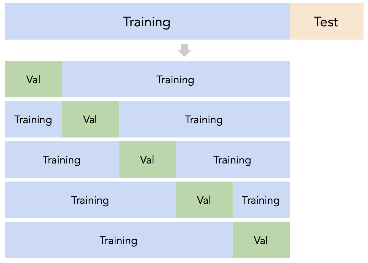
- Since each data point is used for training $k-1$ times and validation once, the (averaged) validation performance should be a good metric of a model's ability to generalize to unseen data.
- $k$-fold cross-validation (or simply "cross-validation") is the technique we will use for finding hyperparameters, or more generally, for choosing between different possible models. It's what you should use in your Portfolio Homework! ✅
Illustrating $k$-fold cross-validation
- To illustrate $k$-fold cross-validation, let's use the following example dataset with $n = 12$ rows.
Suppose this dataset represents our training set, i.e. suppose we already performed a train-test split.
training_data = pd.DataFrame().assign(x=range(0, 120, 10),
                                      y=[9, 1, 58, 3, 6, 4, -2, 8, 1, 10, 1.1, -45])
display_df(training_data, rows=12)
| x | y | |
|---|---|---|
| 0 | 0 | 9.0 |
| 1 | 10 | 1.0 |
| 2 | 20 | 58.0 |
| 3 | 30 | 3.0 |
| 4 | 40 | 6.0 |
| 5 | 50 | 4.0 |
| 6 | 60 | -2.0 |
| 7 | 70 | 8.0 |
| 8 | 80 | 1.0 |
| 9 | 90 | 10.0 |
| 10 | 100 | 1.1 |
| 11 | 110 | -45.0 |
- Suppose we choose $k = 4$. Then, each fold has $\frac{12}{4} = 3$ rows.
show_cv_slides()
$k$-fold cross-validation, in general
- First, shuffle the entire training set randomly and split it into $k$ disjoint folds, or "slices". Then:
- For each hyperparameter:
- For each slice:
- Let the slice be the "validation set", $V$.
- Let the rest of the data be the "training set", $T$.
- Train a model using the selected hyperparameter on the training set $T$.
- Evaluate the model on the validation set $V$.
- Compute the average validation error (e.g. MSE) for the particular hyperparameter.
- For each slice:
- Choose the hyperparameter with the lowest average validation error.
Loading the data
- To illustrate, let's continue using the roughly-cubic dataset titled "Sample 1" from the past few lectures.
np.random.seed(23) # For reproducibility.
def sample_from_pop(n=100):
    x = np.linspace(-2, 3, n)
    y = x ** 3 + (np.random.normal(0, 3, size=n))
    return pd.DataFrame({'x': x, 'y': y})
sample_1 = sample_from_pop()
px.scatter(sample_1, x='x', y='y', title='Sample 1')
- We'll look at how to use $k$-fold cross-validation to choose a polynomial degree that best generalizes to unseen data.
- Before doing cross-validation, we must always perform a train-test split.
from sklearn.model_selection import train_test_split
X_train, X_test, y_train, y_test = train_test_split(sample_1[['x']], sample_1['y'], random_state=23)
$k$-fold cross-validation in sklearn
- The
cross_val_scorefunction insklearnimplements $k$-fold cross-validation for us!
cross_val_score(estimator, X_train, y_train, cv)
from sklearn.model_selection import cross_val_score
- Let's perform $k$-fold cross validation in order to help us pick a degree for polynomial regression from the list [1, 2, ..., 25].
- We'll use $k=5$ since it's a common choice (and the default in
sklearn).
from sklearn.linear_model import LinearRegression
from sklearn.preprocessing import PolynomialFeatures
from sklearn.pipeline import make_pipeline
errs_df = pd.DataFrame()
for d in range(1, 26):
    pl = make_pipeline(PolynomialFeatures(d), LinearRegression())
    # The `scoring` argument is used to specify that we want to compute the MSE;
    # the default is R^2. It's called "neg" MSE because,
    # by default, sklearn likes to "maximize" scores, and maximizing -MSE is the same
    # as minimizing MSE.
    errs = cross_val_score(pl, X_train, y_train,
                           cv=5, scoring='neg_mean_squared_error')
    errs_df[f'Deg {d}'] = -errs # Negate to turn positive (sklearn computed negative MSE).
errs_df.index = [f'Fold {i}' for i in range(1, 6)]
errs_df.index.name = 'Validation Fold'
$k$-fold cross-validation in sklearn
- Note that for each choice of degree (our hyperparameter), we have five MSEs, one for each "fold" of the data. This means that in total, $5 \cdot 25 = 125$ models were trained!
errs_df
| Deg 1 | Deg 2 | Deg 3 | Deg 4 | ... | Deg 22 | Deg 23 | Deg 24 | Deg 25 | |
|---|---|---|---|---|---|---|---|---|---|
| Validation Fold | |||||||||
| Fold 1 | 24.36 | 14.06 | 7.45 | 7.62 | ... | 40.48 | 69.03 | 43.38 | 220.49 |
| Fold 2 | 31.50 | 19.17 | 7.05 | 10.85 | ... | 796.97 | 1446.11 | 2208.78 | 5666.03 |
| Fold 3 | 15.64 | 11.78 | 9.39 | 9.48 | ... | 61.79 | 80.64 | 474.69 | 4620.71 |
| Fold 4 | 25.95 | 17.57 | 9.47 | 9.46 | ... | 12.24 | 12.02 | 11.86 | 15.02 |
| Fold 5 | 11.12 | 4.74 | 4.44 | 4.81 | ... | 8.85 | 8.54 | 8.65 | 8.27 |
5 rows × 25 columns
- Remember, our goal is to choose the degree with the lowest average validation error.
errs_df.mean(axis=0)
Deg 1       21.71
Deg 2       13.46
Deg 3        7.56
           ...
Deg 23     323.27
Deg 24     549.47
Deg 25    2106.10
Length: 25, dtype: float64
fig = errs_df.mean(axis=0).iloc[:18].plot(kind='line', title='Average Validation Error')
fig.update_layout(xaxis_title='Degree', yaxis_title='Average Validation MSE', showlegend=False)
errs_df.mean(axis=0).idxmin()
'Deg 3'
- Note that if we didn't perform $k$-fold cross-validation, but instead just used a single validation set, we may have ended up with a different result:
errs_df.idxmin(axis=1)
Validation Fold
Fold 1     Deg 9
Fold 2     Deg 3
Fold 3     Deg 3
Fold 4    Deg 10
Fold 5     Deg 3
dtype: object
Question 🤔 (Answer at practicaldsc.org/q)
- Suppose you have a training dataset with 1000 rows.
- You want to decide between 20 hyperparameters for a particular model.
- To do so, you perform 10-fold cross-validation.
- How many times is the first row in the training dataset (
X.iloc[0]) used for training a model?
Grid search
An easier approach: GridSearchCV
- Instead of having to
for-loop over possible hyperparameter values, we can letsklearndo the hard work for us, usingGridSearchCV.
GridSearchCVtakes in:- an un-
fitinstance of an estimator, and - a dictionary of hyperparameter values to try,
and performs $k$-fold cross-validation to find the combination of hyperparameters with the best average validation performance.
- an un-
from sklearn.model_selection import GridSearchCV
- Why do you think it's called "grid search"?
Grid searching for the best polynomial degree
- Let's once again aim to fit a polynomial regression model to
X_trainandy_train, taken fromsample_1.
- Here, we want to try values of degree from 1 through 25, so we'll need to specify these values in a dictionary.
# The key names in this dictionary are chosen very carefully.
# They need to be of the format pipelinestep__hyperparametername,
# where pipelinestep is a lowercase version of the step in the pipeline
# that we want to tune, and
# hyperparameter name is the formal name of the hyperparameter (see the documentation).
hyperparams = {
    'polynomialfeatures__degree': range(1, 26)
}
searcher = GridSearchCV(
    make_pipeline(PolynomialFeatures(), LinearRegression()),
    param_grid=hyperparams,
    cv=5, # k = 5.
    scoring='neg_mean_squared_error'
)
searcher
GridSearchCV(cv=5,
             estimator=Pipeline(steps=[('polynomialfeatures',
                                        PolynomialFeatures()),
                                       ('linearregression',
                                        LinearRegression())]),
             param_grid={'polynomialfeatures__degree': range(1, 26)},
             scoring='neg_mean_squared_error')
In a Jupyter environment, please rerun this cell to show the HTML representation or trust the notebook. On GitHub, the HTML representation is unable to render, please try loading this page with nbviewer.org.
GridSearchCV(cv=5,
             estimator=Pipeline(steps=[('polynomialfeatures',
                                        PolynomialFeatures()),
                                       ('linearregression',
                                        LinearRegression())]),
             param_grid={'polynomialfeatures__degree': range(1, 26)},
scoring='neg_mean_squared_error')Pipeline(steps=[('polynomialfeatures', PolynomialFeatures()),
('linearregression', LinearRegression())])PolynomialFeatures()
LinearRegression()
- Like any other estimator,
GridSearchCVinstances need to befit.
searcher.fit(X_train, y_train)
GridSearchCV(cv=5,
             estimator=Pipeline(steps=[('polynomialfeatures',
                                        PolynomialFeatures()),
                                       ('linearregression',
                                        LinearRegression())]),
             param_grid={'polynomialfeatures__degree': range(1, 26)},
             scoring='neg_mean_squared_error')
In a Jupyter environment, please rerun this cell to show the HTML representation or trust the notebook. On GitHub, the HTML representation is unable to render, please try loading this page with nbviewer.org.
GridSearchCV(cv=5,
             estimator=Pipeline(steps=[('polynomialfeatures',
                                        PolynomialFeatures()),
                                       ('linearregression',
                                        LinearRegression())]),
             param_grid={'polynomialfeatures__degree': range(1, 26)},
scoring='neg_mean_squared_error')Pipeline(steps=[('polynomialfeatures', PolynomialFeatures(degree=3)),
('linearregression', LinearRegression())])PolynomialFeatures(degree=3)
LinearRegression()
- Once fit,
searchercan tell us what it found!
searcher.best_params_
{'polynomialfeatures__degree': 3}
-pd.DataFrame(np.vstack([searcher.cv_results_[f'split{i}_test_score'] for i in range(5)]))
| 0 | 1 | 2 | 3 | ... | 21 | 22 | 23 | 24 | |
|---|---|---|---|---|---|---|---|---|---|
| 0 | 24.36 | 14.06 | 7.45 | 7.62 | ... | 40.48 | 69.03 | 43.38 | 220.49 |
| 1 | 31.50 | 19.17 | 7.05 | 10.85 | ... | 796.97 | 1446.11 | 2208.78 | 5666.03 |
| 2 | 15.64 | 11.78 | 9.39 | 9.48 | ... | 61.79 | 80.64 | 474.69 | 4620.71 |
| 3 | 25.95 | 17.57 | 9.47 | 9.46 | ... | 12.24 | 12.02 | 11.86 | 15.02 |
| 4 | 11.12 | 4.74 | 4.44 | 4.81 | ... | 8.85 | 8.54 | 8.65 | 8.27 |
5 rows × 25 columns
searcheris now a fit regression model – there's no need to refit it on the entire training set, since it already did that.
searcher.predict([[4],
                  [-1],
                  [0]])
array([64.1 , -1.28, 0.28])
Another example: Commute times
- We can also use $k$-fold cross-validation to determine which subset of features to use in a linear model that predicts commute times!
np.random.seed(23)
df = pd.read_csv('data/commute-times.csv')
df['day_of_month'] = pd.to_datetime(df['date']).dt.day
df['month'] = pd.to_datetime(df['date']).dt.month_name()
df.head()
| date | day | home_departure_time | home_departure_mileage | ... | work_departure_time_hr | mileage_to_home | day_of_month | month | |
|---|---|---|---|---|---|---|---|---|---|
| 0 | 5/15/2023 | Mon | 2023-05-15 10:49:00 | 15873.0 | ... | 17.17 | 53.0 | 15 | May |
| 1 | 5/16/2023 | Tue | 2023-05-16 07:45:00 | 15979.0 | ... | NaN | NaN | 16 | May |
| 2 | 5/22/2023 | Mon | 2023-05-22 08:27:00 | 50407.0 | ... | 15.90 | 54.0 | 22 | May |
| 3 | 5/23/2023 | Tue | 2023-05-23 07:08:00 | 50535.0 | ... | NaN | NaN | 23 | May |
| 4 | 5/30/2023 | Tue | 2023-05-30 09:09:00 | 50664.0 | ... | 17.12 | 54.0 | 30 | May |
5 rows × 20 columns
- Let's make several candidate pipelines. But first, as always, a train-test split.
# Here, we're letting X_train and X_test keep all of the columns in the DataFrame
# OTHER than 'minutes'.
X_train, X_test, y_train, y_test = train_test_split(df.drop('minutes', axis=1), df['minutes'], random_state=23)
Creating many pipelines
from sklearn.compose import make_column_transformer, make_column_selector
from sklearn.preprocessing import FunctionTransformer, OneHotEncoder
selecter = FunctionTransformer(lambda x: x) # Shortcut to say "keep just these columns."
week_converter = FunctionTransformer(lambda s: 'Week ' + ((s - 1) // 7 + 1).astype(str))
day_of_month_transformer = make_pipeline(week_converter, OneHotEncoder(drop='first')) # From last class.
pipes = {
    'departure_hour only': make_pipeline(
        make_column_transformer((selecter, ['departure_hour'])),
        LinearRegression()
    ),
    'departure_hour + day_of_month': make_pipeline(
        make_column_transformer((selecter, ['departure_hour', 'day_of_month'])),
        LinearRegression()
    ),
    'departure_hour + day OHE': make_pipeline(
        make_column_transformer(
            (selecter, ['departure_hour']),
            (OneHotEncoder(drop='first', handle_unknown='ignore'), ['day'])
        ),
        LinearRegression()
    ),
    'departure_hour + day OHE + month OHE': make_pipeline(
        make_column_transformer(
            (selecter, ['departure_hour']),
            (OneHotEncoder(drop='first', handle_unknown='ignore'), ['day', 'month'])
        ),
        LinearRegression()
    ),
    'departure_hour with poly features + day OHE + month OHE + week': make_pipeline(
        make_column_transformer(
        (PolynomialFeatures(3), ['departure_hour']),
        (OneHotEncoder(drop='first', handle_unknown='ignore'), ['day', 'month']),
        (day_of_month_transformer, ['day_of_month']),
    ),
    LinearRegression())
}
- Here, we won't be able to use
GridSearchCVdirectly, because we're choosing between many different pipelines, not between hyperparameters for a particular pipeline.
results = pd.DataFrame(columns=['Average Training MSE', 'Average Validation MSE'])
for pipe in pipes:
    fitted = GridSearchCV(
        pipes[pipe],
        param_grid={}, # No hyperparameters, but we could have them.
        scoring='neg_mean_squared_error',
        cv=10, # Change this and see what happens!,
        return_train_score=True # So that we can compute training MSEs, too.
    )
    fitted.fit(X_train, y_train)
    results.loc[pipe] = [-fitted.cv_results_['mean_train_score'][0], -fitted.cv_results_['mean_test_score'][0]]
commute_models_summarized = (
    results
    .sort_values('Average Training MSE')
    .plot(kind='barh', barmode='group', width=1000)
    .update_layout(xaxis_title='Mean Squared Error', yaxis_title='Model')
)
commute_models_summarized
- What's the "right" combination of features to choose?
Summary: Generalization
- Split the data into two sets: training and test.
- Use only the training data when designing, training, and tuning the model.
- Use $k$-fold cross-validation to choose hyperparameters and estimate the model's ability to generalize.
- Do not ❌ look at the test data in this step!
- Commit to your final model and train it using the entire training set.
- Test the data using the test data. If the performance (e.g. MSE) is not acceptable, return to step 2.
- Finally, train on all available data and ship the model to production! 🛳
- 🚨 This is the process you should always use! 🚨
Question 🤔 (Answer at practicaldsc.org/q)
What questions do you have?
Regularization
Motivation
- So far, to us, "model complexity" has essentially meant "number of features."
The main hyperparameter we've tuned is polynomial degree. For instance, a polynomial of degree 5 has 5 features – an $x$, $x^2$, $x^3$, $x^4$, and $x^5$ feature.
In the more recent example, we manually created several different pipelines, each of which used different combinations of features from the commute times dataset.
- Once we've created several different candidate models, we've used cross-validation to choose the one that best generalizes to unseen data.
- Another approach: instead of manually choosing which features to include, put some constraint on the optimal parameters, $w_0^*, w_1^*, ..., w_d^*$.
This would save us time from having to think of combinations of features that might be relevant.
- Intuition: The bigger the optimal parameters $w_0^*, w_1^*, ..., w_d^*$ are, the more overfit the model is to the training data.
Why?
Polynomial regression returns!
- Once again, let's try fitting a polynomial model to Sample 1.
X_train, X_test, y_train, y_test = train_test_split(sample_1[['x']], sample_1['y'], random_state=23)
px.scatter(x=X_train['x'], y=y_train, title="Sample 1's Training Data")
- This time, instead of using cross-validation to choose a polynomial degree, let's pick a degree in advance, like 25.
model = make_pipeline(PolynomialFeatures(25), LinearRegression(fit_intercept=False))
model.fit(X_train, y_train)
Pipeline(steps=[('polynomialfeatures', PolynomialFeatures(degree=25)),
                ('linearregression', LinearRegression(fit_intercept=False))])
In a Jupyter environment, please rerun this cell to show the HTML representation or trust the notebook. On GitHub, the HTML representation is unable to render, please try loading this page with nbviewer.org.
Pipeline(steps=[('polynomialfeatures', PolynomialFeatures(degree=25)),
('linearregression', LinearRegression(fit_intercept=False))])PolynomialFeatures(degree=25)
LinearRegression(fit_intercept=False)
fig = px.scatter(x=X_train['x'], y=y_train, title="Sample 1's Training Data")
fig.add_trace(go.Scatter(
    x=X_train['x'].sort_values(),
    y=model.predict(X_train.sort_values('x')),
    mode='lines',
    line=dict(width=4),
    name='Fit Polynomial of Degree 25'
))
- This degree 25 polynomial is clearly overfit to the training data.
- Observe:
sklearnassigned really large values to many features. For instance, we're seeing that the coefficient on $x^{10}$ is 1712.92. This means that if $x$ changes a little, the output is going to change a lot.
pd.Series(model.named_steps['linearregression'].coef_).abs().sort_values(ascending=False).head()
10    1712.92
8     1418.08
9     1405.07
7     1395.33
12    1268.88
dtype: float64
Penalizing large parameters
- Idea: In addition to just minimizing mean squared error, what if we could also try and prevent large parameter values?
Maybe this would lead to less overfitting!
- Previously, we minimized mean squared error to find $\vec{w}_\text{OLS}^*$: $$R_\text{sq}(\vec{w}) = \frac{1}{n} \lVert \vec{y} - X \vec{w} \rVert^2$$ Here, OLS stands for "ordinary least squares."
- Idea: Instead, minimize regularized mean squared error:
- For each $w_j$, we've added a penalty on how large it is! The larger each $w_j$ is, the larger $R_\text{sq-reg}$ will be.
Remember, the goal is to find the $\vec{w}^*$ that minimizes $R_\text{sq-reg}$.
Note that we're not penalizing the intercept term, which doesn't really contribute to overfitting.
Ridge regression
- The specific penalty we've chosen – $w_j^2$ for each $w_j$ – is called $L_2$ regularization.
- Minimizing mean squared error, with $L_2$ regularization, is called ridge regression. The objective function for ridge regression is:
- $\lambda$ is a hyperparameter, which we choose through cross-validation.
- The $\vec{w}_\text{ridge}^*$ that minimizes $R_\text{ridge}(\vec{w})$ is not necessarily the same as $\vec{w}_\text{OLS}^*$, which minimizes $R_\text{sq}(\vec{w})$!
Question 🤔 (Answer at practicaldsc.org/q)
The objective function we minimize to find $\vec{w}_\text{ridge}^*$ in ridge regression is:
$$R_\text{ridge}(\vec{w}) = \frac{1}{n} \lVert \vec{y} - X \vec{w} \rVert^2 + \lambda \sum_{j = 1}^d w_j^2$$$\lambda$ is a hyperparameter, which we choose through cross-validation.
- What if we pick $\lambda = 0$ – what is $\vec{w}_\text{ridge}^*$ then?
- What happens to $\vec{w}_\text{ridge}^*$ as $\lambda \rightarrow \infty$?
- Can $\lambda$ be negative?
Ridge regression, visualized
- As $\lambda$ increases, the penalty on the size of $\vec{w}_\text{ridge}^*$ increases, meaning that each $w_j^*$ inches closer to 0.
An equivalent way of formulating the ridge regression objective function,
$$\text{minimize} \:\:\:\: \frac{1}{n} \lVert \vec{y} - X \vec{w} \rVert^2 + \lambda \sum_{j = 1}^d w_j^2$$
is as a constrained optimization problem:
$$\text{minimize} \:\:\:\:\frac{1}{n} \lVert \vec{y} - X \vec{w} \rVert^2 \text{ such that } \sum_{j = 1}^d w_j^2 \leq Q$$
- $Q$ and $\lambda$ are inversely related: the larger $Q$ is, the less of a penalty we're putting on size of $\vec{w}_\text{ridge}^*$, so the smaller $\lambda$ is.
The exact relationship between $Q$ and $\lambda$ is outside of the scope of this course, as is the proof of this fact. Take IOE 310!
Intuitively:
- The loss surface for just the mean squared error component is in blue.
- The constraint, $\sum_{j = 1}^d w_j^2 \leq Q$, is in green.
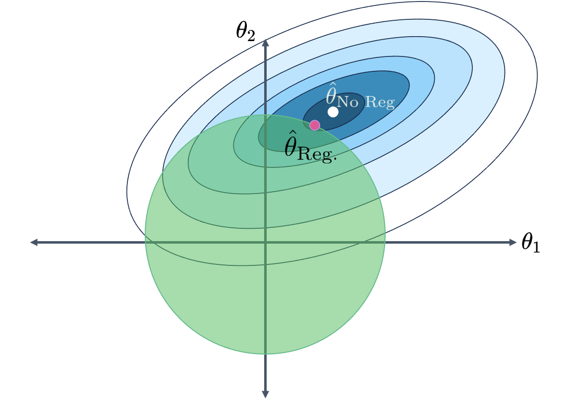 (source)
- The bigger $Q$ is – so, the smaller $\lambda$ is – the larger the green circle is!
- The bigger $Q$ is, the larger the range of possible values for $\vec{w}_\text{ridge}^*$ is, and the closer $\vec{w}_\text{ridge}^*$ gets to $\vec{w}_\text{OLS}^*$.
Finding $\vec{w}_\text{ridge}^*$
- We know that the $\vec{w}_\text{OLS}^*$ that minimizes mean squared error, $$R_\text{sq}(\vec{w}) = \frac{1}{n} \lVert \vec{y} - X \vec{w} \rVert^2$$ is the one that satisfies the normal equations, $X^TX \vec{w} = X^T \vec{y}$.
- Sometimes, $\vec{w}^*_\text{OLS}$ is unique, and sometimes there are infinitely many possible $\vec{w}^*_\text{OLS}$.
There are infinitely many possible $\vec{w}^*_\text{OLS}$ when the design matrix, $X$, is not full rank! All of these infinitely many solutions minimize mean squared error.
- Which vector $\vec{w}_\text{ridge}^*$ minimizes the ridge regression objective function?
- It turns out there is always a unique solution for $\vec{w}_\text{ridge}^*$, even if $X$ is not full rank. It is:
$$\vec{w}_\text{ridge}^* = (X^TX + n \lambda I)^{-1} X^T \vec{y}$$
The proof is outside of the scope of the class, and requires vector calculus.
- Since there is always a unique solution, ridge regression is often used in the presence of multicollinearity!
Taking a step back
- $\vec{w}_\text{ridge}^*$ doesn't minimize mean squared error – it minimizes a slightly different objective function.
- So, why would we use ever use ridge regression?
Ridge regression in sklearn
- Fortunately,
sklearncan perform ridge regression for us.
from sklearn.linear_model import Ridge
- Just to experiment, let's set $\lambda$ to something extremely large and look at the resulting predictions.
# The name of the lambda hyperparameter in sklearn is alpha.
model_large_lambda = make_pipeline(PolynomialFeatures(25), Ridge(alpha=1000000000000000000000000000))
model_large_lambda.fit(X_train, y_train)
fig = px.scatter(x=X_train['x'], y=y_train, title="Sample 1's Training Data")
fig.add_trace(go.Scatter(
    x=X_train['x'].sort_values(),
    y=model_large_lambda.predict(X_train.sort_values('x')),
    mode='lines',
    line=dict(width=4, color='purple'),
    name='Extremely Regularized Polynomial of Degree 25'
))
- What do you notice?
model_large_lambda.named_steps['ridge'].intercept_
3.6606542664388497
y_train.mean()
3.662415381952351
Using GridSearchCV to choose $\lambda$
- In general, we won't just arbitrarily choose a value of $\lambda$.
- Instead, we'll perform $k$-fold cross-validation to choose the $\lambda$ that leads to predictions that work best on unseen test data.
hyperparams = {
    'ridge__alpha': 10.0 ** np.arange(-2, 15) # Try 0.01, 0.1, 1, 10, 100, 1000, ...
}
model_regularized = GridSearchCV(
    estimator=make_pipeline(PolynomialFeatures(25), Ridge()),
    param_grid=hyperparams,
    scoring='neg_mean_squared_error'
)
model_regularized.fit(X_train, y_train)
GridSearchCV(estimator=Pipeline(steps=[('polynomialfeatures',
                                        PolynomialFeatures(degree=25)),
                                       ('ridge', Ridge())]),
             param_grid={'ridge__alpha': array([1.e-02, 1.e-01, 1.e+00, 1.e+01, 1.e+02, 1.e+03, 1.e+04, 1.e+05,
       1.e+06, 1.e+07, 1.e+08, 1.e+09, 1.e+10, 1.e+11, 1.e+12, 1.e+13,
       1.e+14])},
             scoring='neg_mean_squared_error')
In a Jupyter environment, please rerun this cell to show the HTML representation or trust the notebook. On GitHub, the HTML representation is unable to render, please try loading this page with nbviewer.org.
GridSearchCV(estimator=Pipeline(steps=[('polynomialfeatures',
                                        PolynomialFeatures(degree=25)),
                                       ('ridge', Ridge())]),
             param_grid={'ridge__alpha': array([1.e-02, 1.e-01, 1.e+00, 1.e+01, 1.e+02, 1.e+03, 1.e+04, 1.e+05,
       1.e+06, 1.e+07, 1.e+08, 1.e+09, 1.e+10, 1.e+11, 1.e+12, 1.e+13,
       1.e+14])},
scoring='neg_mean_squared_error')Pipeline(steps=[('polynomialfeatures', PolynomialFeatures(degree=25)),
('ridge', Ridge(alpha=1000000000.0))])PolynomialFeatures(degree=25)
Ridge(alpha=1000000000.0)
- Let's check the optimal $\lambda$ it found!
model_regularized.best_params_
{'ridge__alpha': 1000000000.0}
- What do the resulting predictions look like?
# The name of the lambda hyperparameter in sklearn is alpha.
fig = px.scatter(x=X_train['x'], y=y_train, title="Sample 1's Training Data")
fig.add_trace(go.Scatter(
    x=X_train['x'].sort_values(),
    y=model.predict(X_train.sort_values('x')),
    mode='lines',
    line=dict(width=4),
    name='Unregularized Polynomial of Degree 25'
))
fig.add_trace(go.Scatter(
    x=X_train['x'].sort_values(),
    y=model_regularized.predict(X_train.sort_values('x')),
    mode='lines',
    line=dict(width=4, color='green'),
    name='Regularized Polynomial of Degree 25'
))
- It seems that the regularized polynomial is less overfit to the specific noise in the training data than the unregularized polynomial!
- The largest coefficients are all much smaller now, too.
The coefficient on $x^{20}$ is 0.000136.
pd.Series(model_regularized.best_estimator_.named_steps['ridge'].coef_).abs().sort_values(ascending=False).head()
20    1.36e-04
17    1.29e-04
15    8.57e-05
19    8.49e-05
16    5.68e-05
dtype: float64
Another example: Commute times
- Let's use ridge regression to find coefficients for the most complicated commute times model we looked at earlier, to see if it can generalize well to unseen data.
X_train, X_test, y_train, y_test = train_test_split(df.drop('minutes', axis=1), df['minutes'], random_state=23)
- We'll use the model previously labeled
departure_hour with poly features + day OHE + month OHE + week.
commute_models_summarized
Ridge regression for commute times
- Let's first instantiate a Pipeline for the steps we want to execute.
commute_pipe = make_pipeline(
        make_column_transformer(
        (PolynomialFeatures(3), ['departure_hour']),
        (OneHotEncoder(drop='first', handle_unknown='ignore'), ['day', 'month']),
        (day_of_month_transformer, ['day_of_month']),
    ),
    Ridge())
- Then, as before, we'll fit a
GridSearchCVinstance with a hyperparameter grid.
lambdas = 10.0 ** np.arange(-10, 15) # Try 0.00000000001, ..., 1, 10, 100, 1000, ...
hyperparams = {
    'ridge__alpha': lambdas
}
commute_model_regularized = GridSearchCV(
    commute_pipe,
    param_grid = hyperparams,
    scoring='neg_mean_squared_error',
    cv=10
)
commute_model_regularized.fit(X_train, y_train)
GridSearchCV(cv=10,
             estimator=Pipeline(steps=[('columntransformer',
                                        ColumnTransformer(transformers=[('polynomialfeatures',
                                                                         PolynomialFeatures(degree=3),
                                                                         ['departure_hour']),
                                                                        ('onehotencoder',
                                                                         OneHotEncoder(drop='first',
                                                                                       handle_unknown='ignore'),
                                                                         ['day',
                                                                          'month']),
                                                                        ('pipeline',
                                                                         Pipeline(steps=[('functiontransformer',
                                                                                          FunctionTransformer(func=<function <lambda> at 0x177a80820>)),
                                                                                         ('onehotencoder',
                                                                                          OneHotEncoder(drop='first'))]),
                                                                         ['day_of_month'])])),
                                       ('ridge', Ridge())]),
             param_grid={'ridge__alpha': array([1.e-10, 1.e-09, 1.e-08, ..., 1.e+12, 1.e+13, 1.e+14])},
             scoring='neg_mean_squared_error')
In a Jupyter environment, please rerun this cell to show the HTML representation or trust the notebook. On GitHub, the HTML representation is unable to render, please try loading this page with nbviewer.org.
GridSearchCV(cv=10,
             estimator=Pipeline(steps=[('columntransformer',
                                        ColumnTransformer(transformers=[('polynomialfeatures',
                                                                         PolynomialFeatures(degree=3),
                                                                         ['departure_hour']),
                                                                        ('onehotencoder',
                                                                         OneHotEncoder(drop='first',
                                                                                       handle_unknown='ignore'),
                                                                         ['day',
                                                                          'month']),
                                                                        ('pipeline',
                                                                         Pipeline(steps=[('functiontransformer',
                                                                                          FunctionTransformer(func=<function <lambda> at 0x177a80820>)),
                                                                                         ('onehotencoder',
                                                                                          OneHotEncoder(drop='first'))]),
                                                                         ['day_of_month'])])),
                                       ('ridge', Ridge())]),
             param_grid={'ridge__alpha': array([1.e-10, 1.e-09, 1.e-08, ..., 1.e+12, 1.e+13, 1.e+14])},
scoring='neg_mean_squared_error')Pipeline(steps=[('columntransformer',
ColumnTransformer(transformers=[('polynomialfeatures',
                                 PolynomialFeatures(degree=3),
                                 ['departure_hour']),
                                ('onehotencoder',
                                 OneHotEncoder(drop='first',
                                               handle_unknown='ignore'),
                                 ['day', 'month']),
                                ('pipeline',
                                 Pipeline(steps=[('functiontransformer',
                                                  FunctionTransformer(func=<function <lambda> at 0x177a80820>)),
                                                 ('onehotencoder',
                                                  OneHotEncoder(drop='first'))]),
['day_of_month'])])),
('ridge', Ridge())])ColumnTransformer(transformers=[('polynomialfeatures',
PolynomialFeatures(degree=3),
['departure_hour']),
('onehotencoder',
OneHotEncoder(drop='first',
handle_unknown='ignore'),
['day', 'month']),
('pipeline',
Pipeline(steps=[('functiontransformer',
FunctionTransformer(func=<function <lambda> at 0x177a80820>)),
('onehotencoder',
OneHotEncoder(drop='first'))]),
['day_of_month'])])['departure_hour']
PolynomialFeatures(degree=3)
['day', 'month']
OneHotEncoder(drop='first', handle_unknown='ignore')
['day_of_month']
FunctionTransformer(func=<function <lambda> at 0x177a80820>)
OneHotEncoder(drop='first')
Ridge()
- Which $\lambda$ did it choose?
commute_model_regularized.best_params_
{'ridge__alpha': 1.0}
- How did the average validation MSE change with $\lambda$?
Here, large values of $\lambda$ mean less complex models, not more complex.
(
    pd.Series(-commute_model_regularized.cv_results_['mean_test_score'],
              index=np.log(lambdas))
    .to_frame()
    .reset_index()
    .plot(kind='line', x='index', y=0)
    .update_layout(xaxis_title='$\log(\lambda)$', yaxis_title='Average Validation MSE')
)
What's next?
- Could we have chosen a different method of penalizing each $w_j$ other than $w_j^2$?
- Ridge regression's objective function happened to have a closed-form solution. What if we want to minimize a function that can't be minimized by hand?