from lec_utils import *
def sample_from_pop(n=100):
    x = np.linspace(-2, 3, n)
    y = x ** 3 + (np.random.normal(0, 3, size=n))
    return pd.DataFrame({'x': x, 'y': y})
sample_1 = sample_from_pop()

Lecture 18

Feature Engineering, Continued

EECS 398-003: Practical Data Science, Fall 2024

practicaldsc.org • github.com/practicaldsc/fa24

Announcements 📣

• Homework 8 is due on Friday (not today!).
• Homework 7 solutions are available at #259 on Ed.
• Check out the new FAQs page on the course website.
  It has answers to frequently-asked theoretical questions.
• The IA application is out for next semester and is due on Monday! See #238 on Ed for more details.

Come say hi next Thursday!

A few other professors and I are hosting a faculty-student panel, where you can learn more about our career (and personal) paths. Come say hi – there will be pizza 🍕!

RSVP here.

Agenda

• Recap: Multiple linear regression and feature engineering.
• Numerical-to-numerical transformations.
• The modeling recipe, revisited.
• OneHotEncoder and multicollinearity.
• StandardScaler and standardized regression coefficients.

Question 🤔 (Answer at practicaldsc.org/q)

Remember that you can always ask questions anonymously at the link above!

Recap: Multiple linear regression and feature engineering

---

The general problem

• We have $n$ data points, $\left({ \vec x_1}, {y_1}\right), \left({ \vec x_2}, {y_2}\right), \ldots, \left({ \vec x_n}, {y_n}\right)$,

where each $ \vec x_i$ is a feature vector of $d$ features: $${\vec{x_i}} = \begin{bmatrix} {x^{(1)}_i} \\ {x^{(2)}_i} \\ \vdots \\ {x^{(d)}_i} \end{bmatrix}$$

• We want to find a good linear hypothesis function:

$$\begin{align*} H({ \vec x}) &= w_0 + w_1 { x^{(1)}} + w_2 { x^{(2)}} + \ldots + w_d { x^{(d)}}\\ &= \vec w \cdot \text{Aug}({ \vec x}) \end{align*}$$

The general solution

• Define the design matrix $ X \in \mathbb{R}^{n \times (d + 1)}$ and observation vector $ \vec y \in \mathbb{R}^n$:

$${ X= \begin{bmatrix} {1} & { x^{(1)}_1} & { x^{(2)}_1} & \dots & { x^{(d)}_1} \\\\ { 1} & { x^{(1)}_2} & { x^{(2)}_2} & \dots & { x^{(d)}_2} \\\\ \vdots & \vdots & \vdots & & \vdots \\\\ { 1} & { x^{(1)}_n} & { x^{(2)}_n} & \dots & { x^{(d)}_n} \end{bmatrix} = \begin{bmatrix} \text{Aug}({\vec{x_1}})^T \\\\ \text{Aug}({\vec{x_2}})^T \\\\ \vdots \\\\ \text{Aug}({\vec{x_n}})^T \end{bmatrix}} \qquad { \vec y = \begin{bmatrix} { y_1} \\ { y_2} \\ \vdots \\ { y_n} \end{bmatrix}}$$

• Then, solve the normal equations to find the optimal parameter vector, $\vec{w}^*$:

  $${ X^TX} \vec{w}^* = { X^T} { \vec y}$$

The goal of feature engineering

• Feature engineering is the act of finding transformations that transform data into effective quantitative variables.
  Put simply: feature engineering is creating new features using existing features.

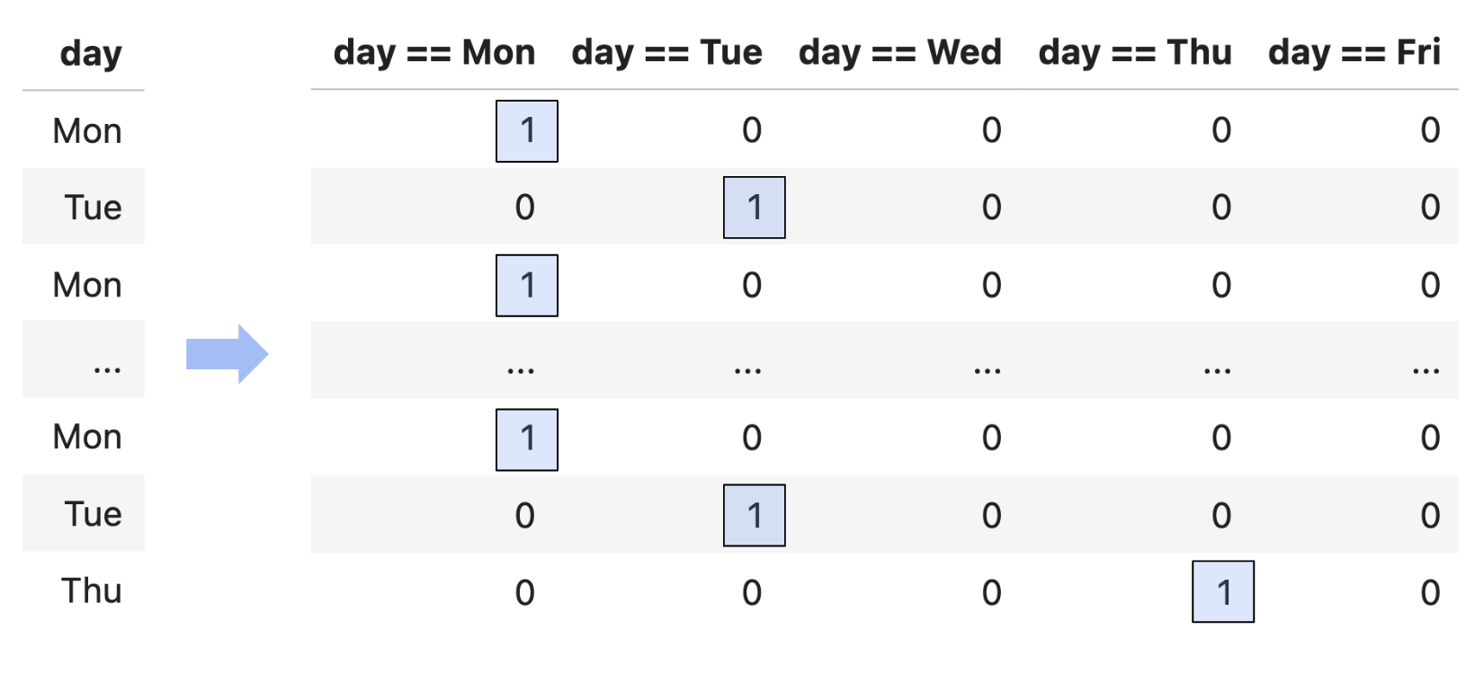
• Example: One hot encoding.

• Example: Numerical-to-numerical transformations.

Numerical-to-numerical transformations

---

Linearization

• The Tukey Mosteller Bulge Diagram helps us pick which numerical-to-numerical transformations to apply to data in order to linearize it.
  Alternative interpretation: it helps us determine which features to create.

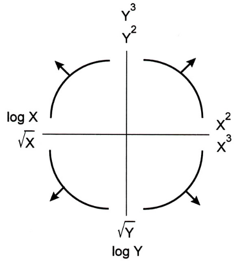
• Why? We're working with linear models. The more linear our data looks in terms of its features, the better we'll able to model the data.

Example: Polynomial regression

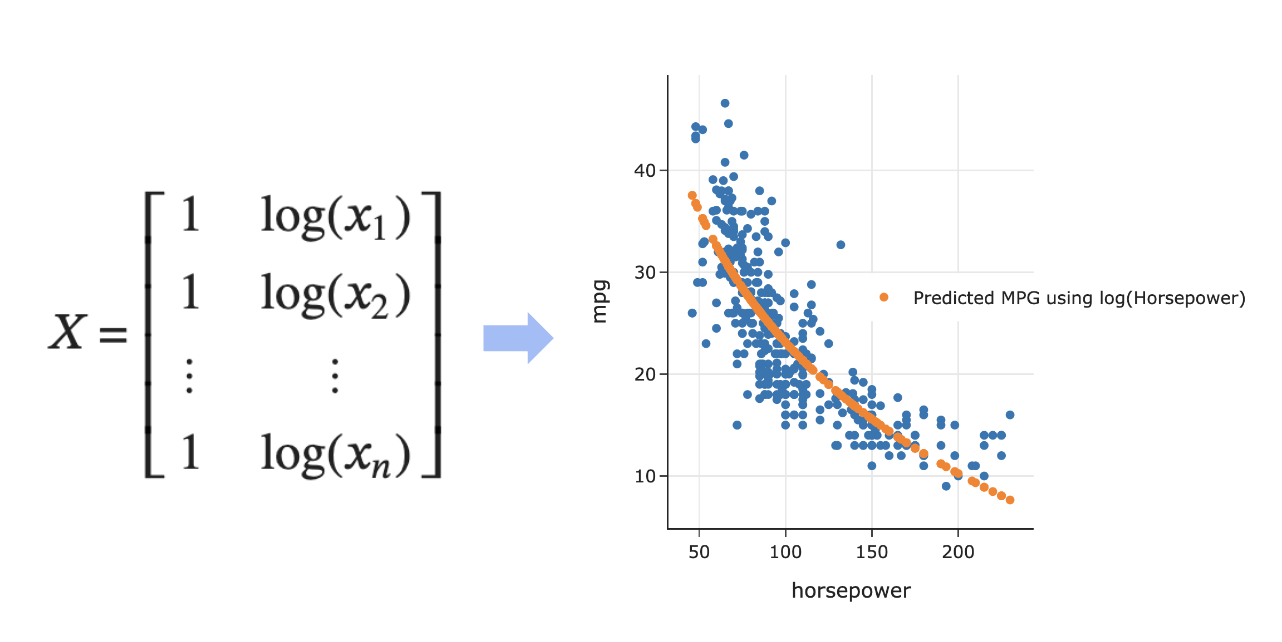
• Last class, we engineered a new feature by taking the $\log$ of an existing feature; this is a numerical-to-numerical transformation.
  This allowed us to create a curve of best fit.

• Consider the dataset below.
  sample_1 is defined at the top of this notebook.

px.scatter(sample_1, x='x', y='y')

• A simple linear regression line isn't sufficient enough to model the relationship between the two variables.

Example: Polynomial regression

• The scatter plot appears to roughly resemble a degree 3 (cubic) polynomial, so let's try and fit a degree 3 polynomial. This will involve creating a design matrix with quadratic and cubic features.

$$H(x) = w_0 + w_1x + w_2x^2 + w_3x^3$$

X = sample_1[['x']].copy()
X

	x
0	-2.00
1	-1.95
2	-1.90
...	...
97	2.90
98	2.95
99	3.00

100 rows × 1 columns

# Note that X itself is not the design matrix;
# sklearn's LinearRegression object will create the needed design matrix
# by adding a column of 1s to the start of X.
X['x^2'] = X['x'] ** 2
X['x^3'] = X['x'] ** 3
X

	x	x^2	x^3
0	-2.00	4.00	-8.00
1	-1.95	3.80	-7.41
2	-1.90	3.61	-6.85
...	...	...	...
97	2.90	8.40	24.36
98	2.95	8.70	25.66
99	3.00	9.00	27.00

100 rows × 3 columns

• Now, let's fit a LinearRegression model from sklearn and look at the resulting predictions.

from sklearn.linear_model import LinearRegression

model = LinearRegression()
model.fit(X=X, y=sample_1['y'])

LinearRegression()

In a Jupyter environment, please rerun this cell to show the HTML representation or trust the notebook.
On GitHub, the HTML representation is unable to render, please try loading this page with nbviewer.org.

model.predict(X)

array([-9.72, -9.03, -8.38, ..., 24.1 , 25.47, 26.89])

fig = px.scatter(sample_1, x='x', y='y')
fig.add_trace(go.Scatter(
    x=X['x'],
    y=model.predict(X),
    mode='lines',
    line=dict(width=5),
    name='Degree 3 Polynomial of Best Fit'
))

• The orange curve above is of the form:

$$H^*(x) = -0.38 - 0.49x + 0.12x^2 + 1.05x^3$$

model.intercept_

-0.5198355347237897

model.coef_

array([-0.31, -0.21,  1.12])

• While the curve is non-linear, it is linear in the parameters.

Reference Slide

Example: Amdahl's Law

• Amdahl's Law relates the runtime of a program on $p$ processors to the time to do the sequential and nonsequential parts on one processor.

$$\displaystyle H(p) = t_\text{S} + \frac{t_\text{NS}}{p}$$

• Collect data by timing a program with varying numbers of processors:

Processors	Time (Hours)
1	8
2	4
4	3

---

• To find $w_0^*$ and $w_1^*$ in the hypothesis function $H(x) = w_0 + w_1 \cdot \frac{1}{x}$, we need to create an appropriate design matrix:

$$X = \begin{bmatrix} 1 & \frac{1}{1} \\ 1 & \frac{1}{2} \\ 1 & \frac{1}{4} \end{bmatrix}$$

• Then, the problem reduces to finding the parameter vector, $\vec{w}^*$, that solves the normal equations, $(X^TX)^{-1}X^T \vec{y}$.

Question 🤔 (Answer at practicaldsc.org/q)

Which hypothesis function is not linear in the parameters?

• A. $H(\vec{x}) = w_1 (x^{(1)} x^{(2)}) + \frac{w_2}{x^{(1)}} \sin \left( x^{(2)} \right)$
• B. $H(\vec{x}) = 2^{w_1} x^{(1)}$
• C. $H(\vec{x}) = \vec{w} \cdot \text{Aug}(\vec{x})$
• D. $H(\vec{x}) = w_1 \cos (x^{(1)}) + w_2 2^{x^{(2)} \log x^{(3)}}$
• E. More than one of the above.

How do we fit hypothesis functions that aren't linear in the parameters?

• Suppose we want to fit the hypothesis function:

$$H(x) = w_0 e^{w_1 x}$$

• This is not linear in terms of $w_0$ and $w_1$, so our results for linear regression don't apply.

• Possible solution: Try to transform the above equation so that it is linear in some other parameters, by applying an operation to both sides.

$$H(x) = w_0 e^{w_1 x}$$

• Suppose we take the $\log$ of both sides of the equation.

$$\log H(x) = \log (w_0 e^{w_1x})$$

• Then, using properties of logarithms, we have:

$$\log H(x) = \underbrace{\log(w_0)}_{\text{this is just a constant!}} + w_1 x$$

• Solution: Create a new hypothesis function, $T(x)$, with parameters $b_0$ and $b_1$, where $T(x) = b_0 + b_1 x$.

• This hypothesis function is related to $H(x)$ by the relationship $T(x) = \log H(x)$.

• $\vec{b}$ is related to $\vec{w}$ by $b_0 = \log w_0$ and $b_1 = w_1$.

• Our new observation vector, $\vec{z}$, is $\begin{bmatrix} \log y_1 \\ \log y_2 \\ ... \\ \log y_n \end{bmatrix}$.

• $T(x) = b_0 + b_1x$ is linear in its parameters, $b_0$ and $b_1$.

• Use the solution to the normal equations to find $\vec{b}^*$, and the relationship between $\vec{b}$ and $\vec{w}$ to find $\vec{w}^*$.

The modeling recipe, revisited

---

The original modeling recipe, from Lecture 14

1. Choose a model.

2. Choose a loss function.

3. Minimize average loss to find optimal model parameters.

The updated modeling recipe

0. Create, or engineer, features to best reflect the "meaning" behind data.
   Recently, we've done this with one hot encoding and numerical-to-numerical transformations.

1. Choose a model.
   Recently, we've used the simple/multiple linear regression model.

2. Choose a loss function.
   Recently, we've mostly used squared loss.

3. Minimize average loss (empirical risk) to find optimal model parameters, $\vec{w}^*$.
   Originally, we had to use calculus or linear algebra to minimize empirical risk, but more recently we've just used model.fit. This step is also called fitting the model to the data.

4. Evaluate the performance of the model in relation to other models, using MSE or $R^2$.

• We can do all of the above directly in sklearn!

preprocessing and linear_models

• For the feature engineering step of the modeling pipeline, we will use sklearn's preprocessing module.

• For the model creation step of the modeling pipeline, we will use sklearn's linear_model module, as we've already seen. linear_model.LinearRegression is an example of an estimator class.

Transformer classes

• Transformers take in "raw" data and output "processed" data. They are used for creating features.

• Transformers, like most relevant features of sklearn, are classes, not functions, meaning you need to instantiate them and call their methods.

• Today, we'll introduce two transformer classes. We'll look at how to write code to use each one, but also discuss some of the underlying statistical nuances.

• Next class, we'll see how to chain transformers and estimators together into larger Pipelines.

OneHotEncoder and multicollinearity

---

Example: Commute times 🚗

• For this first example, we'll continue working with our commute times dataset.

df = pd.read_csv('data/commute-times.csv')
df['day_of_month'] = pd.to_datetime(df['date']).dt.day
df['month'] = pd.to_datetime(df['date']).dt.month_name()
df.head()

	date	day	home_departure_time	home_departure_mileage	...	work_departure_time_hr	mileage_to_home	day_of_month	month
0	5/15/2023	Mon	2023-05-15 10:49:00	15873.0	...	17.17	53.0	15	May
1	5/16/2023	Tue	2023-05-16 07:45:00	15979.0	...	NaN	NaN	16	May
2	5/22/2023	Mon	2023-05-22 08:27:00	50407.0	...	15.90	54.0	22	May
3	5/23/2023	Tue	2023-05-23 07:08:00	50535.0	...	NaN	NaN	23	May
4	5/30/2023	Tue	2023-05-30 09:09:00	50664.0	...	17.12	54.0	30	May

5 rows × 20 columns

• We'll focus specifically on the 'day' and 'month' columns.

df[['day', 'month']]

	day	month
0	Mon	May
1	Tue	May
2	Mon	May
...	...	...
62	Mon	March
63	Tue	March
64	Thu	March

65 rows × 2 columns

Example transformer: OneHotEncoder

• Last class, we had to manually one hot encode the 'day' column. Let's figure out how to one hot encode it automatically, along with the new 'month' column.

df[['day', 'month']]

	day	month
0	Mon	May
1	Tue	May
2	Mon	May
...	...	...
62	Mon	March
63	Tue	March
64	Thu	March

65 rows × 2 columns

• First, we need to import the relevant class from sklearn.preprocessing.
  It's best practice to import just the relevant classes you need from sklearn.

from sklearn.preprocessing import OneHotEncoder

• Like an estimator, we need to instantiate and fit our OneHotEncoder instsance before it can transform anything.

ohe = OneHotEncoder()

# Error!
ohe.transform(df[['day', 'month']])

---------------------------------------------------------------------------
NotFittedError                            Traceback (most recent call last)
Cell In[16], line 2
      1 # Error!
----> 2 ohe.transform(df[['day', 'month']])

File ~/miniforge3/envs/pds/lib/python3.10/site-packages/sklearn/utils/_set_output.py:313, in _wrap_method_output.<locals>.wrapped(self, X, *args, **kwargs)
    311 @wraps(f)
    312 def wrapped(self, X, *args, **kwargs):
--> 313     data_to_wrap = f(self, X, *args, **kwargs)
    314     if isinstance(data_to_wrap, tuple):
    315         # only wrap the first output for cross decomposition
    316         return_tuple = (
    317             _wrap_data_with_container(method, data_to_wrap[0], X, self),
    318             *data_to_wrap[1:],
    319         )

File ~/miniforge3/envs/pds/lib/python3.10/site-packages/sklearn/preprocessing/_encoders.py:1008, in OneHotEncoder.transform(self, X)
    985 def transform(self, X):
    986     """
    987     Transform X using one-hot encoding.
    988 
   (...)
   1006         returned.
   1007     """
-> 1008     check_is_fitted(self)
   1009     transform_output = _get_output_config("transform", estimator=self)["dense"]
   1010     if transform_output != "default" and self.sparse_output:

File ~/miniforge3/envs/pds/lib/python3.10/site-packages/sklearn/utils/validation.py:1661, in check_is_fitted(estimator, attributes, msg, all_or_any)
   1658     raise TypeError("%s is not an estimator instance." % (estimator))
   1660 if not _is_fitted(estimator, attributes, all_or_any):
-> 1661     raise NotFittedError(msg % {"name": type(estimator).__name__})

NotFittedError: This OneHotEncoder instance is not fitted yet. Call 'fit' with appropriate arguments before using this estimator.

# Need to fit first.
ohe.fit(df[['day', 'month']])

OneHotEncoder()

In a Jupyter environment, please rerun this cell to show the HTML representation or trust the notebook.
On GitHub, the HTML representation is unable to render, please try loading this page with nbviewer.org.

• Once we've fit, when we use the transform method, we get a result we might not expect.

ohe.transform(df[['day', 'month']])

<65x16 sparse matrix of type '<class 'numpy.float64'>'
	with 130 stored elements in Compressed Sparse Row format>

• Since the resulting matrix is sparse – most of its elements are 0 – sklearn uses a more efficient representation than a regular numpy array. We can convert to a regular (dense) array:

ohe.transform(df[['day', 'month']]).toarray()

array([[0., 1., 0., ..., 0., 0., 0.],
       [0., 0., 0., ..., 0., 0., 0.],
       [0., 1., 0., ..., 0., 0., 0.],
       ...,
       [0., 1., 0., ..., 0., 0., 0.],
       [0., 0., 0., ..., 0., 0., 0.],
       [0., 0., 1., ..., 0., 0., 0.]])

• The column names from df[['day', 'month']] don't appear in the output above. We can use the get_feature_names_out method on ohe to access the names and order of the one hot encoded columns, though:

ohe.get_feature_names_out()

array(['day_Fri', 'day_Mon', 'day_Thu', 'day_Tue', 'day_Wed',
       'month_August', 'month_December', 'month_February',
       'month_January', 'month_July', 'month_June', 'month_March',
       'month_May', 'month_November', 'month_October', 'month_September'],
      dtype=object)

pd.DataFrame(ohe.transform(df[['day', 'month']]).toarray(), 
             columns=ohe.get_feature_names_out()) # If we need a DataFrame back, for some reason.

	day_Fri	day_Mon	day_Thu	day_Tue	...	month_May	month_November	month_October	month_September
0	0.0	1.0	0.0	0.0	...	1.0	0.0	0.0	0.0
1	0.0	0.0	0.0	1.0	...	1.0	0.0	0.0	0.0
2	0.0	1.0	0.0	0.0	...	1.0	0.0	0.0	0.0
...	...	...	...	...	...	...	...	...	...
62	0.0	1.0	0.0	0.0	...	0.0	0.0	0.0	0.0
63	0.0	0.0	0.0	1.0	...	0.0	0.0	0.0	0.0
64	0.0	0.0	1.0	0.0	...	0.0	0.0	0.0	0.0

65 rows × 16 columns

• Usually, we won't perform all of these intermediate steps, since the OneHotEncoder will be part of a larger Pipeline.

Example: Heights and weights

• We now know how to use OneHotEncoder.

• To illustrate a mathematical issue involving one hot encoding, let's load in another dataset, this time containing the weights and heights of 25,000 18 year olds, taken from here.

people = pd.read_csv('data/heights-weights.csv').drop(columns=['Index'])
people.head()

	Height (Inches)	Weight (Pounds)
0	65.78	112.99
1	71.52	136.49
2	69.40	153.03
3	68.22	142.34
4	67.79	144.30

people.plot(kind='scatter', x='Height (Inches)', y='Weight (Pounds)', 
            title='Weight vs. Height for 25,000 18 Year Olds')

Motivating example

• Suppose we fit a simple linear regression model that uses height in inches to predict weight in pounds.

$$\text{predicted weight (pounds)} = w_0 + w_1 \cdot \text{height (inches)}$$

X = people[['Height (Inches)']]
y = people['Weight (Pounds)']

people_one_feat = LinearRegression()
people_one_feat.fit(X, y)

LinearRegression()

In a Jupyter environment, please rerun this cell to show the HTML representation or trust the notebook.
On GitHub, the HTML representation is unable to render, please try loading this page with nbviewer.org.

• $w_0^*$ and $w_1^*$ are shown below, along with the model's MSE on the data we used to train it.
  We call this the model's training MSE.

people_one_feat.intercept_, people_one_feat.coef_

(-82.57574306454093, array([3.08]))

from sklearn.metrics import mean_squared_error
mean_squared_error(y, people_one_feat.predict(X))

101.58853248632849

An added feature

• Now, suppose we fit another regression model, that uses height in inches AND height in centimeters to predict weight.

$$\text{predicted weight (pounds)} = w_0 + w_1 \cdot \text{height (inches)} + w_2 \cdot \text{height (cm)}$$

people['Height (cm)'] = people['Height (Inches)'] * 2.54 # 1 inch = 2.54 cm.

X2 = people[['Height (Inches)', 'Height (cm)']]

people_two_feat = LinearRegression()
people_two_feat.fit(X2, y)

LinearRegression()

In a Jupyter environment, please rerun this cell to show the HTML representation or trust the notebook.
On GitHub, the HTML representation is unable to render, please try loading this page with nbviewer.org.

• What are $w_0^*$, $w_1^*$, $w_2^*$, and the model's MSE?

people_two_feat.intercept_, people_two_feat.coef_

(-82.57525639659859, array([ 3.38e+10, -1.33e+10]))

mean_squared_error(y, people_two_feat.predict(X2))

101.58853251653949

• Observation: The intercept is the same as before (roughly -82.57), as is the MSE. However, the coefficients on 'Height (Inches)' and 'Height (cm)' are massive in size!

• It should be unsurprising that the MSE is the same, because the span of the design matrix is the same. So, the best predictions should be the same, too.

• But what's going on with the coefficients?

Redundant features

• Let's use simpler numbers for illustration. Suppose in the first model, $w_0^* = -80$ and $w_1^* = 3$.

$$\text{predicted weight (pounds)} = -80 + 3 \cdot \text{height (inches)}$$

• In the second model, we have:

$$\begin{align*}\text{predicted weight (pounds)} &= w_0^* + w_1^* \cdot \text{height (inches)} + w_2^* \cdot \text{height (cm)} \\ &= w_0^* + w_1^* \cdot \text{height (inches)} + w_2^* \cdot \big( 2.54^* \cdot \text{height (inches)} \big) \\ &= w_0^* + \left(w_1^* + 2.54 \cdot w_2^* \right) \cdot \text{height (inches)} \end{align*}$$

• In the first model, we already found the "best" intercept ($-80$) and slope ($3$) in a linear model that uses height in inches to predict weight.

• So, as long as $w_1^* + 2.54 \cdot w_2^* = 3$ in the second model, the second model's predictions will be the same as the first, and hence they will also minimize MSE.

Infinitely many parameter choices

• Issue: There are an infinite number of $w_1^*$ and $w_2^*$ that satisfy $w_1^* + 2.54 \cdot w_2^* = 3$!

$$\text{predicted weight} = -80 - 10 \cdot \text{height (inches)} + \frac{13}{2.54} \cdot \text{height (cm)}$$

$$\text{predicted weight} = -80 + 10 \cdot \text{height (inches)} - \frac{7}{2.54} \cdot \text{height (cm)}$$

• Both hypothesis functions look very different, but actually make the same predictions.

• model.coef_ could return either set of coefficients, or any other of the infinitely many options.

• But neither set of coefficients is has any meaning!

(-80 - 10 * people.iloc[:, 0] + (13 / 2.54) * people.iloc[:, 2]).head()

0    117.35
1    134.55
2    128.20
3    124.65
4    123.36
dtype: float64

(-80 + 10 * people.iloc[:, 0] - (7 / 2.54) * people.iloc[:, 2]).head()

0    117.35
1    134.55
2    128.20
3    124.65
4    123.36
dtype: float64

Multicollinearity

• Multicollinearity occurs when features in a regression model are highly correlated with one another.
  In other words, multicollinearity occurs when a feature can be predicted using a linear combination of other features, fairly accurately.

• When multicollinearity is present in the features, the coefficients in the model are uninterpretable – they have no meaning.
  A "slope" represents "the rate of change of $y$ with respect to a feature", when all other features are held constant – but if there's multicollinearity, you can't hold other features constant.

• Note: Multicollinearity doesn't impact a model's predictions!
  • It doesn't impact a model's ability to generalize to unseen data.
  • If features are multicollinear in the data we've seen, they will probably be multicollinear in the data we haven't seen, drawn from the same distribution.

• Solutions:
  • Manually remove highly correlated features.
  • Use a dimensionality reduction technique (such as PCA) to automatically reduce dimensions.

One hot encoding and multicollinearity

• One hot encoding will result in multicollinearity unless you drop one of the one hot encoded features.

• Suppose we have the following fitted model:
  For illustration, assume 'weekend' was originally a categorical feature with two possible values, 'Yes' or 'No'.

$$ \begin{aligned} H(x) = 1 + 2 \cdot (\text{weekend==Yes}) - 2 \cdot (\text{weekend==No}) \end{aligned} $$

• This is equivalent to:

$$ \begin{aligned} H(x) = 10 - 7 \cdot (\text{weekend==Yes}) - 11 \cdot (\text{weekend==No}) \end{aligned} $$

• Note that for a particular row in the dataset, $\text{weekend==Yes} + \text{weekend==No}$ is always equal to 1.

• This means that the columns of the design matrix, $X$, for this model is not linearly independent, since the column of all 1s can be written as a linear combination of the $\text{weekend==Yes}$ and $\text{weekend==No}$ columns.

• This means that the design matrix is not full rank, which means that $X^TX$ is not invertible.

• This means that there are infinitely many possible solutions $\vec{w}^*$ to the normal equations, $(X^TX) \vec{w} = X^T\vec{y}$!
  That's a problem, because we don't know which of these infinitely many solutions model.coef_ will find for us, and it's impossible to interpret the resulting coefficients, as we saw on the last slide.

• Solution: Drop one of the one hot encoded columns. OneHotEncoder has an option to do this.

OneHotEncoder returns

• Let's switch back to the commute times dataset, df.

df[['day', 'month']]

	day	month
0	Mon	May
1	Tue	May
2	Mon	May
...	...	...
62	Mon	March
63	Tue	March
64	Thu	March

65 rows × 2 columns

• Let's try using drop='first' when instantiating a OneHotEncoder.

ohe_drop_one = OneHotEncoder(drop='first')

ohe_drop_one.fit(df[['day', 'month']])

OneHotEncoder(drop='first')

In a Jupyter environment, please rerun this cell to show the HTML representation or trust the notebook.
On GitHub, the HTML representation is unable to render, please try loading this page with nbviewer.org.

• How many features did the resulting transformer create?

len(ohe_drop_one.get_feature_names_out())

14

• Where did this number come from?

df['day'].nunique()

5

df['month'].nunique()

11

Key takeaways

• Multicollinearity is present in a linear model when one feature can be accurately predicted using one or more other features.
  In other words, it is present when a feature is redundant.

• Multicollinearity doesn't pose an issue for prediction; it doesn't hinder a model's ability to generalize. Instead, it renders the coefficients of a linear model meaningless.

StandardScaler and standardized regression coefficients

---

Example: Predicting sales 📈

• To illustrate the next transformer class, we'll introduce a new dataset.

sales = pd.read_csv('data/sales.csv')
sales.head()

	net_sales	sq_ft	inventory	advertising	district_size	competing_stores
0	231.0	3.0	294	8.2	8.2	11
1	156.0	2.2	232	6.9	4.1	12
2	10.0	0.5	149	3.0	4.3	15
3	519.0	5.5	600	12.0	16.1	1
4	437.0	4.4	567	10.6	14.1	5

• For each of 26 stores, we have:
  • net sales,
  • square feet,
  • inventory,
  • advertising expenditure,
  • district size, and
  • number of competing stores.

• Our goal is to predict 'net_sales' as a function of other features.

An initial model

sales.head()

	net_sales	sq_ft	inventory	advertising	district_size	competing_stores
0	231.0	3.0	294	8.2	8.2	11
1	156.0	2.2	232	6.9	4.1	12
2	10.0	0.5	149	3.0	4.3	15
3	519.0	5.5	600	12.0	16.1	1
4	437.0	4.4	567	10.6	14.1	5

• No transformations are needed to predict 'net_sales'.

sales_model = LinearRegression()
sales_model.fit(X=sales.iloc[:, 1:], y=sales.iloc[:, 0])

LinearRegression()

In a Jupyter environment, please rerun this cell to show the HTML representation or trust the notebook.
On GitHub, the HTML representation is unable to render, please try loading this page with nbviewer.org.

• Suppose we're interested in learning how the various features impact 'net_sales', rather than just predicting 'net_sales' for a new store. We'd then look at the coefficients.

sales_model.coef_

array([16.2 ,  0.17, 11.53, 13.58, -5.31])

pd.DataFrame().assign(
    column=sales.columns[1:],
    original_coef=sales_model.coef_,
).set_index('column')

	original_coef
column
sq_ft	16.20
inventory	0.17
advertising	11.53
district_size	13.58
competing_stores	-5.31

• What do you notice?

sales.iloc[:, 1:]

	sq_ft	inventory	advertising	district_size	competing_stores
0	3.0	294	8.2	8.2	11
1	2.2	232	6.9	4.1	12
2	0.5	149	3.0	4.3	15
...	...	...	...	...	...
24	3.5	382	9.8	11.5	5
25	5.1	590	12.0	15.7	0
26	8.6	517	7.0	12.0	8

27 rows × 5 columns

Which features are most "important"?

• The most important feature is not necessarily the feature with largest magnitude coefficient, because different features may be on different scales.

• Suppose I fit two hypothesis functions:
  • $H_1$ has store size measured in square feet.
  • $H_2$ has store size measured in square meters.

• Store size is just as important in both hypothesis functions.

• But 1 square meter $\approx 10.76$ square feet, so the sizes in square meters will be 10.76x smaller.

• So, the coefficient of store size in $H_2$ will be 10.76 times larger than the coefficient of store size in $H_1$.
  Intuition: if the values themselves are smaller, you need to multiply them by bigger coefficients to get the same predictions!

• Solution: If you care about the interpretability of the resulting coefficients, standardize each feature before performing regression.

Standardization

• Recall: to standardize a feature $x_1, x_2, ..., x_n$, we use the formula: $$z(x_i) = \frac{x_i - \bar{x}}{\sigma_x}$$

• Example: 1, 7, 7, 9.

  • Mean: $\frac{1 + 7 + 7 + 9}{4} = \frac{24}{4} = 6$.
  • Standard deviation:

  $$\text{SD} = \sqrt{\frac{1}{4} \left( (1-6)^2 + (7-6)^2 + (7-6)^2 + (9-6)^2 \right)} = \sqrt{\frac{1}{4} \cdot 36} = 3$$

  • Standardized data:

  $$1 \mapsto \frac{1-6}{3} = \boxed{-\frac{5}{3}} \qquad 7 \mapsto \frac{7-6}{3} = \boxed{\frac{1}{3}} \qquad 7 \mapsto \boxed{\frac{1}{3}} \qquad 9 \mapsto \frac{9-6}{3} = \boxed{1}$$

Example transformer: StandardScaler

• StandardScaler standardizes data using the mean and standard deviation of the data, as described on the previous slide.

• Like OneHotEncoder, StandardScaler requires some knowledge (mean and SD) of the dataset before transforming, so we need to fit an StandardScaler transformer before we can use the transform method.

from sklearn.preprocessing import StandardScaler
stdscaler = StandardScaler()

# This is like saying "determine the mean and SD of each column in sales, 
# other than the 'net_sales' column".
stdscaler.fit(sales.iloc[:, 1:])

StandardScaler()

In a Jupyter environment, please rerun this cell to show the HTML representation or trust the notebook.
On GitHub, the HTML representation is unable to render, please try loading this page with nbviewer.org.

• Now, we can standardize any dataset, using the mean and standard deviation of the columns in sales.iloc[:, 1:]. Typical usage is to fit transformer on a sample and use that already-fit transformer to transform future data.

stdscaler.transform([[5, 300, 10, 15, 6]])

/Users/surajrampure/miniforge3/envs/pds/lib/python3.10/site-packages/sklearn/base.py:493: UserWarning:

X does not have valid feature names, but StandardScaler was fitted with feature names

array([[ 0.85, -0.47,  0.51,  1.05, -0.36]])

stdscaler.transform(sales.iloc[:, 1:].tail(5))

array([[-1.13, -1.31, -1.35, -1.6 ,  0.89],
       [ 0.14,  0.39,  0.4 ,  0.32, -0.36],
       [ 0.09, -0.03,  0.46,  0.36, -0.57],
       [ 0.9 ,  1.08,  1.05,  1.19, -1.61],
       [ 2.67,  0.69, -0.3 ,  0.46,  0.05]])

• We can peek under the hood and see what it computed!

stdscaler.mean_

array([  3.33, 387.48,   8.1 ,   9.69,   7.74])

stdscaler.var_

array([    3.89, 35191.58,    13.72,    25.44,    23.08])

• If needed, the fit_transform method will fit the transformer and then transform the data in one go.

new_scaler = StandardScaler()

new_scaler.fit_transform(sales.iloc[:, 1:].tail(5))

array([[-1.33, -1.79, -1.71, -1.88,  1.48],
       [-0.32,  0.28,  0.43,  0.19, -0.05],
       [-0.36, -0.24,  0.49,  0.23, -0.31],
       [ 0.29,  1.11,  1.22,  1.13, -1.58],
       [ 1.71,  0.64, -0.43,  0.34,  0.46]])

• Why are the values above different from the values in stdscaler.transform(sales.iloc[:, 1:].tail(5))?

Interpreting standardized regression coefficients

• Now that we have a technique for standardizing the feature columns of sales, let's fit a new regression object.

sales_model_std = LinearRegression()
sales_model_std.fit(X=stdscaler.transform(sales.iloc[:, 1:]),
                    y=sales.iloc[:, 0])

LinearRegression()

In a Jupyter environment, please rerun this cell to show the HTML representation or trust the notebook.
On GitHub, the HTML representation is unable to render, please try loading this page with nbviewer.org.

• Let's now look at the resulting coefficients, and compare them to the coefficients before we standardized.

pd.DataFrame().assign(
    column=sales.columns[1:],
    original_coef=sales_model.coef_,
    standardized_coef=sales_model_std.coef_
).set_index('column')

	original_coef	standardized_coef
column
sq_ft	16.20	31.97
inventory	0.17	32.76
advertising	11.53	42.69
district_size	13.58	68.50
competing_stores	-5.31	-25.52

• Did the performance of the resulting model change?

mean_squared_error(sales.iloc[:, 0],
                   sales_model.predict(sales.iloc[:, 1:]))

242.27445717154964

mean_squared_error(sales.iloc[:, 0],
                   sales_model_std.predict(stdscaler.transform(sales.iloc[:, 1:])))

242.27445717154956

• No!
  The span of the design matrix did not change, so the predictions did not change. It's just the coefficients that changed.

Key takeaways

• The result of standardizing each feature (separately!) is that the units of each feature are on the same scale.
  • There's no need to standardize the outcome ('net_sales' here), since it's not being compared to anything.
  • Also, we can't standardize the column of all 1s.

• Then, solve the normal equations. The resulting $w_0^*, w_1^*, \ldots, w_d^*$ are called the standardized regression coefficients.

• Standardized regression coefficients can be directly compared to one another.

• As we saw on the previous slide, standardizing each feature does not change the MSE of the resulting hypothesis function!

StandardScaler summary

Property	Example	Description
Initialize with parameters	stdscaler = StandardScaler()	z-score the data (no parameters)
Fit the transformer	stdscaler.fit(X)	Compute the mean and SD of X
Transform data in a dataset	feat = stdscaler.transform(X_new)	z-score X_new with mean and SD of X
Fit and transform	stdscaler.fit_transform(X)	Compute the mean and SD of X, then z-score X

What's next?

• Even though we have a OneHotEncoder transformer object, to actually use one hot encoding to make predictions, we need to:
  • Manually instantiate a OneHotEncoder object, and then fit it.
  • Create a new design matrix by taking the result of calling transform on the OneHotEncoder object and concatenating other relevant numerical columns.
  • Manually instantiate a LinearRegression object, and then fit it using the result of the above step.

• As we build more and more sophisticated models, it will be challenging to keep track of all of these individual steps ourselves.

• As such, we often build Pipelines.