from lec_utils import *

Lecture 17

Multiple Linear Regression and Feature Engineering

EECS 398-003: Practical Data Science, Fall 2024

practicaldsc.org • github.com/practicaldsc/fa24

Announcements 📣

• Homework 8 is due on Friday (not Thursday!).
• Homework 7 solutions are available at #259 on Ed.
• Check out the new FAQs page on the course website.
  It has answers to frequently-asked theoretical questions.
• The IA application is out for next semester and is due on Monday! See #238 on Ed for more details.

Agenda

• Recap: Regression and linear algebra.
• Multiple linear regression.
• Regression in sklearn.
• Feature engineering.
• Example: Horsepower 🚗.

Today's lecture is back to being in a notebook, but is still quite math heavy.

Question 🤔 (Answer at practicaldsc.org/q)

Remember that you can always ask questions anonymously at the link above!

Recap: Regression and linear algebra

---

Terminology recap

• Define the design matrix $\color{#007aff} X \in \mathbb{R}^{n \times 2}$, observation vector $\color{orange} \vec{y} \in \mathbb{R}^n$, and parameter vector $\vec{w} \in \mathbb{R}^2$ as:

$${\color{#007aff} {X} = \begin{bmatrix} {\color{#007aff} 1} & {\color{#007aff} x_1} \\ {\color{#007aff} 1} & {\color{#007aff} x_2} \\ \vdots & \vdots \\ {\color{#007aff} 1} & {\color{#007aff} x_n} \end{bmatrix}} \qquad {\color{orange} \vec{y} = \begin{bmatrix} y_1 \\ y_2 \\ \vdots \\ y_n \end{bmatrix}} \qquad \vec{w} = \begin{bmatrix} w_0 \\ w_1 \end{bmatrix}$$

• Our goal is to find the $\vec w^*$ that minimizes $R_\text{sq}(\vec{w}) = \frac{1}{n} \lVert {\color{orange} \vec{y}} - {\color{#007aff} X}\vec{w} \rVert^2$.

• Last lecture, we showed that the best $\vec w^*$ is one that satisfies the normal equations:

$${\color{#007aff} X^TX} \vec{w}^* = {\color{#007aff} X^T} {\color{orange} \vec y}$$

• If ${\color{#007aff} X^TX}$ is invertible, there's a unique solution for $\vec w^*$:

$$\vec w^* = ({\color{#007aff}{X^TX}})^{-1} {\color{#007aff}{X^T}}\color{orange}\vec{y}$$

• We chose $\vec{w}^*$ so that ${\color{purple} \vec h^*} = {\color{#007aff} X} \vec{w}^*$ is the projection of $\color{orange} \vec{y}$ onto the span of the columns of the design matrix, $\color{#007aff}X$.

The optimal parameter vector, $\vec{w}^*$

• To find the optimal model parameters for simple linear regression, $w_0^*$ and $w_1^*$, we previously minimized $R_\text{sq}(w_0, w_1) = \frac{1}{n} \sum_{i = 1}^n ({\color{orange} y_i} - (w_0 + w_1 {\color{#007aff} x_i}))^2$.

• We found, using calculus, that:
  • $\boxed{w_1^* = \frac{\sum_{i = 1}^n (x_i - \bar{x})(y_i - \bar{y})}{\sum_{i = 1}^n (x_i - \bar{x})^2} = r \frac{\sigma_y}{\sigma_x}}$.
  • $\boxed{w_0^* = \bar{y} - w_1^* \bar{x}}$.

• Another way of finding optimal model parameters for simple linear regression is to find the $\vec{w}^*$ that minimizes $R_\text{sq}(\vec{w}) = \frac{1}{n} \lVert {\color{orange} \vec{y}} - {\color{#007aff} X}\vec{w} \rVert^2$.

• The minimizer, if ${\color{#007aff}{X^TX}}$ is invertible, is the vector $\boxed{\vec{w}^* = ({\color{#007aff}{X^TX}})^{-1} {\color{#007aff}{X^T}}\color{orange}\vec{y}}$.
  If not, solve the normal equations from the previous slide.

• These $\boxed{\text{formulas}}$ are equivalent!

Multiple linear regression

---

So far, we've fit simple linear regression models, which use only one feature ('departure_hour') for making predictions.

Incorporating multiple features

• In the context of the commute times dataset, the simple linear regression model we fit was of the form:

$$\begin{align*}\text{pred. commute} &= H(\text{departure hour}) \\ &= w_0 + w_1 \cdot \text{departure hour} \end{align*}$$

• Now, we'll try and fit a multiple linear regression model of the form:

$$\begin{align*}\text{pred. commute} &= H(\text{departure hour, day of month}) \\ &= w_0 + w_1 \cdot \text{departure hour} + w_2 \cdot \text{day of month} \end{align*}$$

• Linear regression with multiple features is called multiple linear regression.

• How do we find $w_0^*$, $w_1^*$, and $w_2^*$?

Geometric interpretation

• The hypothesis function:

  $$H(\text{departure hour}) = w_0 + w_1 \cdot \text{departure hour}$$

  looks like a line in 2D.

• Questions:

  • How many dimensions do we need to graph the hypothesis function:

  $$H(\text{departure hour, day of month}) = w_0 + w_1 \cdot \text{departure hour} + w_2 \cdot \text{day of month}$$

  • What is the shape of the hypothesis function?

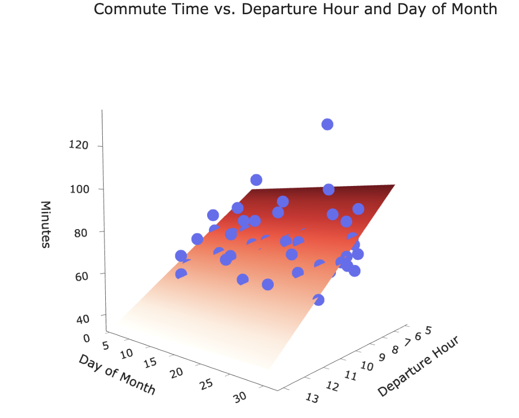
Our new hypothesis function is a plane in 3D!
Our goal is to find the plane of best fit that pierces through the cloud of points.

The hypothesis vector

• When our hypothesis function is of the form:

  $$H(\text{departure hour}) = w_0 + w_1 \cdot \text{departure hour} + w_2 \cdot \text{day of month}$$

  the hypothesis vector $\color{purple} \vec{h} \in \mathbb{R}^n$ can be written as:

$${\color{purple} \vec{h}} = \begin{bmatrix} H(\text{departure hour}_1, \text{day}_1) \\ H(\text{departure hour}_2, \text{day}_2) \\ ... \\ H(\text{departure hour}_n, \text{day}_n) \\ \end{bmatrix} = \begin{bmatrix} 1 & \text{departure hour}_1 & \text{day}_1 \\ 1 & \text{departure hour}_2 & \text{day}_2 \\ ... & ... & ... \\ 1 & \text{departure hour}_n & \text{day}_n \end{bmatrix} \begin{bmatrix} w_0 \\ w_1 \\ w_2 \end{bmatrix} $$

Finding the optimal parameters

• To find the optimal parameter vector, $\vec{w}^*$, we can use the design matrix $\color{#007aff} X \in \mathbb{R}^{n \times 3}$ and observation vector $\color{orange} \vec y \in \mathbb{R}^n$:

$${\color{#007aff} X = \begin{bmatrix} 1 & \text{departure hour}_1 & \text{day}_1 \\ 1 & \text{departure hour}_2 & \text{day}_2 \\ ... & ... & ... \\ 1 & \text{departure hour}_n & \text{day}_n \end{bmatrix}} \qquad {\color{orange} \vec{y} = \begin{bmatrix} \text{commute time}_1 \\ \text{commute time}_2 \\ \vdots \\ \text{commute time}_n \end{bmatrix}}$$

• Then, all we need to do is solve the normal equations once again:

  $${\color{#007aff} X^TX} \vec{w}^* = {\color{#007aff} X^T} {\color{orange} \vec y}$$

  If ${\color{#007aff} X^TX}$ is invertible, we know the solution is:

$$\vec{w}^* = ({\color{#007aff}{X^TX}})^{-1} {\color{#007aff}{X^T}}\color{orange}\vec{y}$$

• Let's generalize this notion beyond just two features.

Notation for multiple linear regression

• We will need to keep track of multiple features for every individual in our dataset.
  In practice, we could have hundreds, millions, or billions of features!

• As before, subscripts distinguish between individuals in our dataset. We have $n$ individuals, also called training examples.

• Superscripts distinguish between features. We have $d$ features.

  $$\text{departure hour:} \:\: \color{#007aff}x^{(1)}$$

  $$\text{day of month:} \:\: \color{#007aff}x^{(2)}$$

  Think of $\color{#007aff} x^{(1)}$, $\color{#007aff}x^{(2)}$, ... as new variable names, like new letters.

Feature vectors

• Suppose we have the following dataset.

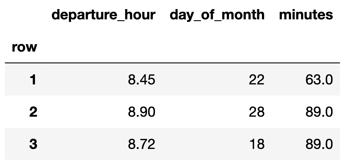
• We can represent each day with a feature vector, $\color{#007aff} \vec{x} = \begin{bmatrix} x^{(1)} \\ x^{(2)} \end{bmatrix}$:

$$\color{#007aff} \vec x_1 = \begin{bmatrix} 8.45 \\ 22 \end{bmatrix} \qquad \vec x_2 = \begin{bmatrix} 8.90 \\ 28 \end{bmatrix} \qquad \vec x_2 = \begin{bmatrix} 8.72 \\ 18 \end{bmatrix}$$

Augmented feature vectors

• The augmented feature vector $\text{Aug}({\color{#007aff}\vec x})$ is the vector obtained by adding a 1 to the front of feature vector $\color{#007aff} \vec x$:

$$ {\color{#007aff} \vec x = \begin{bmatrix} {\color{#007aff}x^{(1)}} \\ {\color{#007aff}x^{(2)}} \\ \vdots \\ {\color{#007aff}x^{(d)}} \end{bmatrix} \qquad \text{Aug}({\color{#007aff} \vec x}) = \begin{bmatrix} 1 \\ {\color{#007aff}x^{(1)}} \\ {\color{#007aff}x^{(2)}} \\ \vdots \\ {\color{#007aff} x^{(d)}} \end{bmatrix}} \qquad \vec w = \begin{bmatrix} w_0 \\ w_1 \\ w_2\\ \vdots \\ w_d \end{bmatrix} $$

• For example, if $\color{#007aff} \vec x_1 = \begin{bmatrix} 8.45 \\ 22 \end{bmatrix}$, then $\text{Aug}({\color{#007aff} \vec x_1}) = {\color{#007aff} \begin{bmatrix} 1 \\ 8.45 \\ 22 \end{bmatrix}}$.

• Then, our hypothesis function for a single data point is:

$$\begin{align*} H({\color{#007aff} \vec x}) &= w_0 + w_1 {\color{#007aff} x^{(1)}} + w_2 {\color{#007aff} x^{(2)}} + \ldots + w_d {\color{#007aff} x^{(d)}}\\ &= \vec w \cdot \text{Aug}({\color{#007aff} \vec x}) \end{align*}$$

The general problem

• We have $n$ data points, $\left({\color{#007aff} \vec x_1}, {\color{orange}y_1}\right), \left({\color{#007aff} \vec x_2}, {\color{orange}y_2}\right), \ldots, \left({\color{#007aff} \vec x_n}, {\color{orange}y_n}\right)$,

where each $\color{#007aff} \vec x_i$ is a feature vector of $d$ features: $${\color{#007aff}\vec{x_i}} = \begin{bmatrix} {\color{#007aff}x^{(1)}_i} \\ {\color{#007aff}x^{(2)}_i} \\ \vdots \\ {\color{#007aff}x^{(d)}_i} \end{bmatrix}$$

• We want to find a good linear hypothesis function:

$$\begin{align*} H({\color{#007aff} \vec x}) &= w_0 + w_1 {\color{#007aff} x^{(1)}} + w_2 {\color{#007aff} x^{(2)}} + \ldots + w_d {\color{#007aff} x^{(d)}}\\ &= \vec w \cdot \text{Aug}({\color{#007aff} \vec x}) \end{align*}$$

The general solution

• Define the design matrix $ X \in \mathbb{R}^{n \times (d + 1)}$ and observation vector $\color{orange} \vec y \in \mathbb{R}^n$:

$${\color{#007aff} X= \begin{bmatrix} {1} & { x^{(1)}_1} & { x^{(2)}_1} & \dots & { x^{(d)}_1} \\\\ { 1} & { x^{(1)}_2} & { x^{(2)}_2} & \dots & { x^{(d)}_2} \\\\ \vdots & \vdots & \vdots & & \vdots \\\\ { 1} & { x^{(1)}_n} & { x^{(2)}_n} & \dots & { x^{(d)}_n} \end{bmatrix} = \begin{bmatrix} \text{Aug}({\vec{x_1}})^T \\\\ \text{Aug}({\vec{x_2}})^T \\\\ \vdots \\\\ \text{Aug}({\vec{x_n}})^T \end{bmatrix}} \qquad {\color{orange} \vec y = \begin{bmatrix} {\color{orange} y_1} \\ {\color{orange} y_2} \\ \vdots \\ {\color{orange} y_n} \end{bmatrix}}$$

• Then, solve the normal equations to find the optimal parameter vector, $\vec{w}^*$:

  $${\color{#007aff} X^TX} \vec{w}^* = {\color{#007aff} X^T} {\color{orange} \vec y}$$

Note on parameters

• With $d$ features, $\vec w$ has $d+1$ entries.

• Again, $\vec w^*$ represents our optimal parameter vector, that minimizes mean squared error.

• $w_0^*$ is the bias, also known as the intercept.

• $w_1^*, w_2^*, ... , w_d^*$ each give the weight, or coefficient, or slope, of a feature.

$$H^*({\color{#007aff} \vec x}) = w_0^* + w_1^* {\color{#007aff} x^{(1)}} + w_2^* {\color{#007aff} x^{(2)}} + \ldots + w_d^* {\color{#007aff} x^{(d)}}$$

Question 🤔 (Answer at practicaldsc.org/q)

Remember that you can always ask questions anonymously at the link above!

Regression in sklearn

Loading the data

• Run the cell below to load in our commute times dataset.

df = pd.read_csv('data/commute-times.csv')
df['day_of_month'] = pd.to_datetime(df['date']).dt.day
df.head()

	date	day	home_departure_time	home_departure_mileage	...	minutes_to_home	work_departure_time_hr	mileage_to_home	day_of_month
0	5/15/2023	Mon	2023-05-15 10:49:00	15873.0	...	72.0	17.17	53.0	15
1	5/16/2023	Tue	2023-05-16 07:45:00	15979.0	...	NaN	NaN	NaN	16
2	5/22/2023	Mon	2023-05-22 08:27:00	50407.0	...	82.0	15.90	54.0	22
3	5/23/2023	Tue	2023-05-23 07:08:00	50535.0	...	NaN	NaN	NaN	23
4	5/30/2023	Tue	2023-05-30 09:09:00	50664.0	...	76.0	17.12	54.0	30

5 rows × 19 columns

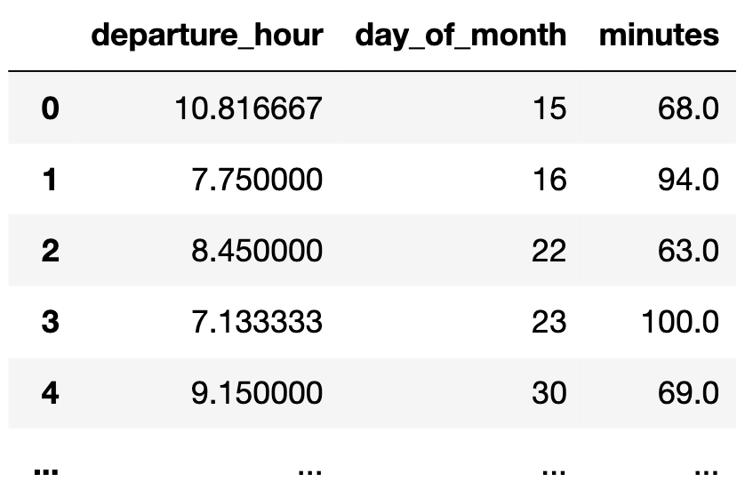
• For now, the only relevant columns for us are 'departure_hour', 'day_of_month', and 'minutes'.

df[['departure_hour', 'day_of_month', 'minutes']]

	departure_hour	day_of_month	minutes
0	10.82	15	68.0
1	7.75	16	94.0
2	8.45	22	63.0
...	...	...	...
62	7.58	4	68.0
63	7.45	5	90.0
64	7.60	7	83.0

65 rows × 3 columns

sklearn

• sklearn (scikit-learn) implements many common steps in the feature and model creation pipeline.
  It is widely used throughout industry and academia.

• It interfaces with numpy arrays, and to an extent, pandas DataFrames.

• Huge benefit: the documentation online is excellent.

The LinearRegression class

• sklearn comes with several subpackages, including linear_model and tree, each of which contains several classes of models.

• We'll start with the LinearRegression class from linear_model.

from sklearn.linear_model import LinearRegression

• Important: From the documentation, we have:

LinearRegression fits a linear model with coefficients w = (w1, …, wp) to minimize the residual sum of squares between the observed targets in the dataset, and the targets predicted by the linear approximation.

In other words, **`LinearRegression` minimizes mean squared error by default**! (Per the documentation, it also includes an intercept term by default.)

LinearRegression?

Init signature:
LinearRegression(
    *,
    fit_intercept=True,
    copy_X=True,
    n_jobs=None,
    positive=False,
)
Docstring:     
Ordinary least squares Linear Regression.

LinearRegression fits a linear model with coefficients w = (w1, ..., wp)
to minimize the residual sum of squares between the observed targets in
the dataset, and the targets predicted by the linear approximation.

Parameters
----------
fit_intercept : bool, default=True
    Whether to calculate the intercept for this model. If set
    to False, no intercept will be used in calculations
    (i.e. data is expected to be centered).

copy_X : bool, default=True
    If True, X will be copied; else, it may be overwritten.

n_jobs : int, default=None
    The number of jobs to use for the computation. This will only provide
    speedup in case of sufficiently large problems, that is if firstly
    `n_targets > 1` and secondly `X` is sparse or if `positive` is set
    to `True`. ``None`` means 1 unless in a
    :obj:`joblib.parallel_backend` context. ``-1`` means using all
    processors. See :term:`Glossary <n_jobs>` for more details.

positive : bool, default=False
    When set to ``True``, forces the coefficients to be positive. This
    option is only supported for dense arrays.

    .. versionadded:: 0.24

Attributes
----------
coef_ : array of shape (n_features, ) or (n_targets, n_features)
    Estimated coefficients for the linear regression problem.
    If multiple targets are passed during the fit (y 2D), this
    is a 2D array of shape (n_targets, n_features), while if only
    one target is passed, this is a 1D array of length n_features.

rank_ : int
    Rank of matrix `X`. Only available when `X` is dense.

singular_ : array of shape (min(X, y),)
    Singular values of `X`. Only available when `X` is dense.

intercept_ : float or array of shape (n_targets,)
    Independent term in the linear model. Set to 0.0 if
    `fit_intercept = False`.

n_features_in_ : int
    Number of features seen during :term:`fit`.

    .. versionadded:: 0.24

feature_names_in_ : ndarray of shape (`n_features_in_`,)
    Names of features seen during :term:`fit`. Defined only when `X`
    has feature names that are all strings.

    .. versionadded:: 1.0

See Also
--------
Ridge : Ridge regression addresses some of the
    problems of Ordinary Least Squares by imposing a penalty on the
    size of the coefficients with l2 regularization.
Lasso : The Lasso is a linear model that estimates
    sparse coefficients with l1 regularization.
ElasticNet : Elastic-Net is a linear regression
    model trained with both l1 and l2 -norm regularization of the
    coefficients.

Notes
-----
From the implementation point of view, this is just plain Ordinary
Least Squares (scipy.linalg.lstsq) or Non Negative Least Squares
(scipy.optimize.nnls) wrapped as a predictor object.

Examples
--------
>>> import numpy as np
>>> from sklearn.linear_model import LinearRegression
>>> X = np.array([[1, 1], [1, 2], [2, 2], [2, 3]])
>>> # y = 1 * x_0 + 2 * x_1 + 3
>>> y = np.dot(X, np.array([1, 2])) + 3
>>> reg = LinearRegression().fit(X, y)
>>> reg.score(X, y)
1.0
>>> reg.coef_
array([1., 2.])
>>> reg.intercept_
3.0...
>>> reg.predict(np.array([[3, 5]]))
array([16.])
File:           ~/miniforge3/envs/pds/lib/python3.10/site-packages/sklearn/linear_model/_base.py
Type:           ABCMeta
Subclasses:     

Fitting a multiple linear regression model

• Let's aim to use sklearn to find the optimal parameters for the following model:

  $$\text{predicted commute time} = w_0 + w_1 \cdot \text{departure hour} + w_2 \cdot \text{day of month}$$

• First, we must instantiate a LinearRegression object and fit it. By calling fit, we are saying "minimize mean squared error on this dataset and find $w^*$."

model_multiple = LinearRegression()
# Note that there are two arguments to fit – X and y!
# (It is not necessary to write X= and y=)
model_multiple.fit(X=df[['departure_hour', 'day_of_month']], y=df['minutes'])

LinearRegression()

In a Jupyter environment, please rerun this cell to show the HTML representation or trust the notebook.
On GitHub, the HTML representation is unable to render, please try loading this page with nbviewer.org.

• After fitting, we can access $w^*$ – that is, the best intercept and coefficients.

model_multiple.intercept_, model_multiple.coef_ 

(141.86402699471932, array([-8.22,  0.06]))

• These coefficients tell us that the "best way" (according to squared loss) to make commute time predictions using a linear model is using:

$$\text{predicted commute time} = 141.86 - 8.22 \cdot \text{departure hour} + 0.06 \cdot \text{day of month}$$

• This is the plane of best fit given historical data; it is not a causal statement.

• Let's visualize this model, as we did in Lecture 16.

XX, YY = np.mgrid[5:14:1, 0:31:1]
Z = model_multiple.intercept_ + model_multiple.coef_[0] * XX + model_multiple.coef_[1] * YY
plane = go.Surface(x=XX, y=YY, z=Z, colorscale='Reds')
fig = go.Figure(data=[plane])
fig.add_trace(go.Scatter3d(x=df['departure_hour'], 
                           y=df['day_of_month'], 
                           z=df['minutes'], mode='markers', marker = {'color': '#656DF1'}))
fig.update_layout(scene=dict(xaxis_title='Departure Hour',
                             yaxis_title='Day of Month',
                             zaxis_title='Minutes'),
                  title='Commute Time vs. Departure Hour and Day of Month',
                  width=1000, height=500)

Making predictions

• Fit LinearRegression objects also have a predict method, which can be used to predict commute times given a 'departure_hour' and 'day_of_month'.

# What if I leave at 9:15AM on the 26th of the month?
model_multiple.predict([[9.25, 26]]) 

/Users/surajrampure/miniforge3/envs/pds/lib/python3.10/site-packages/sklearn/base.py:493: UserWarning:

X does not have valid feature names, but LinearRegression was fitted with feature names

array([67.26])

# Since we trained on a DataFrame, the input to model_multiple.predict should also
# be a DataFrame. To avoid having to do this, we can use .to_numpy()
# when specifying X= and y=.
model_multiple.predict(pd.DataFrame({'departure_hour': [9.25], 'day_of_month': [26]}))

array([67.26])

Comparing models

• Since we're going to start to fit lots of different models to the commute times dataset, it'll be useful to compare their mean squared errors.

• sklearn has a built-in mean_squared_error function.
  Remember, the units of MSE are the units of $y$, squared. So the value below is 96.78 $\text{minutes}^2$.

from sklearn.metrics import mean_squared_error

mean_squared_error(df['minutes'], model_multiple.predict(df[['departure_hour', 'day_of_month']])) 

96.78730488437492

• Let's construct a dictionary to keep track of the MSEs we've seen so far.

mse_dict = {}
mse_dict['departure_hour + day_of_month'] = mean_squared_error(df['minutes'], model_multiple.predict(df[['departure_hour', 'day_of_month']]))

• To compare, let's also fit and measure a simple linear model and constant model.

# Simple linear model.
model_simple = LinearRegression()
model_simple.fit(X=df[['departure_hour']], y=df['minutes'])
mse_dict['departure_hour'] = mean_squared_error(df['minutes'], model_simple.predict(df[['departure_hour']]))

# Constant model.
model_constant = df['minutes'].mean()
mse_dict['constant'] = mean_squared_error(df['minutes'], np.ones(df.shape[0]) * model_constant)

• As we can see, adding 'day_of_month' as a feature barely reduced our model's MSE.
  Next week, when we learn about generalization, we'll see why sometimes adding more features is a bad thing!

mse_dict

{'departure_hour + day_of_month': 96.78730488437492,
 'departure_hour': 97.04687150819183,
 'constant': 167.535147928994}

The .score method of a LinearRegression object

• Model objects in sklearn that have already been fit have a score method.

model_multiple.score(df[['departure_hour', 'day_of_month']], df['minutes']) 

0.4222865704252339

• That doesn't look like the RMSE... what is it? 🤔

Aside: $R^2$

• $R^2$, pronounced "coefficient of determination" or "multiple R-squared", is a measure of the quality of a linear fit.

• There are a few equivalent ways of computing it, assuming your model is linear and has an intercept term:

$$R^2 = \frac{\text{var}(\text{predicted $y$ values})}{\text{var}(\text{actual $y$ values})}$$$$R^2 = \left[ \text{correlation}(\text{predicted $y$ values}, \text{actual $y$ values}) \right]^2$$

• Interpretation: $R^2$ is the proportion of variance in $y$ that the linear model explains.

• In the simple linear regression case, it is the square of the correlation coefficient, $r$.

• Key idea: $R^2$ ranges from 0 to 1. The closer it is to 1, the better the linear fit is.
  Just like $r$, $R^2$ has no units of measurement. This is unlike MSE, which has the units of $y$, squared.

Reference Slide

Calculating $R^2$

• Let's calculate the $R^2$ for model_multiple's predictions in three different ways.

pred = df.assign(predicted=model_multiple.predict(df[['departure_hour', 'day_of_month']]))
pred

	date	day	home_departure_time	home_departure_mileage	...	work_departure_time_hr	mileage_to_home	day_of_month	predicted
0	5/15/2023	Mon	2023-05-15 10:49:00	15873.0	...	17.17	53.0	15	53.76
1	5/16/2023	Tue	2023-05-16 07:45:00	15979.0	...	NaN	NaN	16	79.03
2	5/22/2023	Mon	2023-05-22 08:27:00	50407.0	...	15.90	54.0	22	73.61
...	...	...	...	...	...	...	...	...	...
62	3/4/2024	Mon	2024-03-04 07:35:00	39120.0	...	17.27	52.0	4	79.73
63	3/5/2024	Tue	2024-03-05 07:27:00	59161.0	...	17.28	55.0	5	80.88
64	3/7/2024	Thu	2024-03-07 07:36:00	59270.0	...	NaN	NaN	7	79.76

65 rows × 20 columns

• Method 1: $R^2 = \frac{\text{var}(\text{predicted $y$ values})}{\text{var}(\text{actual $y$ values})}$.

np.var(pred['predicted']) / np.var(pred['minutes'])

0.42228657042523415

• Method 2: $R^2 = \left[ \text{correlation}(\text{predicted $y$ values}, \text{actual $y$ values}) \right]^2$.
  Note: By correlation here, we are referring to $r$, the same correlation coefficient we saw last week.

np.corrcoef(pred['predicted'], pred['minutes'])[0, 1] ** 2

0.4222865704252346

• Method 3: LinearRegression.score.

model_multiple.score(df[['departure_hour', 'day_of_month']], df['minutes'])

0.4222865704252339

• All three methods provide the same result!

Relationship between $R^2$ and MSE

• For linear models with an intercept term,

$$R^2 = 1 - \frac{\text{MSE}}{\text{var}(\text{actual $y$ values})}$$

1 - mean_squared_error(pred['minutes'], pred['predicted']) / np.var(pred['minutes'])

0.42228657042523376

LinearRegression class summary

Property	Example	Description
Initialize model parameters	lr = LinearRegression()	Create (empty) linear regression model
Fit the model to the data	lr.fit(X, y)	Determines regression coefficients
Use model for prediction	lr.predict(X_new)	Uses regression line to make predictions
Evaluate the model	lr.score(X, y)	Calculates the $R^2$ of the LR model
Access model attributes	lr.coef_, lr.intercept_	Accesses the regression coefficients and intercept

What's next?

• So far, in our journey to predict 'minutes', we've only used two numerical features in our dataset, 'departure_hour' and 'day_of_month'.

df[['departure_hour', 'day_of_month', 'minutes']]

	departure_hour	day_of_month	minutes
0	10.82	15	68.0
1	7.75	16	94.0
2	8.45	22	63.0
...	...	...	...
62	7.58	4	68.0
63	7.45	5	90.0
64	7.60	7	83.0

65 rows × 3 columns

• There's a lot of information in df that we didn't use –'day', for example. We can't use these 'day' in it's current form as it's non-numeric.

• How do we use categorical features in a regression model?

Feature engineering ⚙️

The goal of feature engineering

• Feature engineering is the act of finding transformations that transform data into effective quantitative variables.

• A feature function $\phi$ (phi, pronounced "fea") is a mapping from raw data to $d$-dimensional space, i.e. $\phi: \text{raw data} \rightarrow \mathbb{R}^d$.
  If two observations $x_i$ and $x_j$ are "similar" in the raw data space, then $\phi(x_i)$ and $\phi(x_j)$ should also be "similar."

• A "good" choice of features depends on many factors:
  • The kind of data, i.e. quantitative, ordinal, or nominal.
  • The relationship(s) being modeled.
  • The model type, e.g. linear models, decision tree models, neural networks.

One hot encoding

• One hot encoding is a transformation that turns a categorical feature into several binary features.

• Suppose a column has $N$ unique values, $A_1$, $A_2$, ..., $A_N$. For each unique value $A_i$, we define the following feature function:

$$\phi_i(x) = \left\{\begin{array}{ll}1 & {\rm if\ } x == A_i \\ 0 & {\rm if\ } x\neq A_i \\ \end{array}\right. $$

• Note that 1 means "yes" and 0 means "no".

• One hot encoding is also called "dummy encoding", and $\phi(x)$ may also be referred to as an "indicator variable".

Example: One hot encoding 'day'

• For each unique value of 'day' in our dataset, we must create a column for just that 'day'.

df.head()

	date	day	home_departure_time	home_departure_mileage	...	minutes_to_home	work_departure_time_hr	mileage_to_home	day_of_month
0	5/15/2023	Mon	2023-05-15 10:49:00	15873.0	...	72.0	17.17	53.0	15
1	5/16/2023	Tue	2023-05-16 07:45:00	15979.0	...	NaN	NaN	NaN	16
2	5/22/2023	Mon	2023-05-22 08:27:00	50407.0	...	82.0	15.90	54.0	22
3	5/23/2023	Tue	2023-05-23 07:08:00	50535.0	...	NaN	NaN	NaN	23
4	5/30/2023	Tue	2023-05-30 09:09:00	50664.0	...	76.0	17.12	54.0	30

5 rows × 19 columns

df['day'].value_counts()

day
Tue    25
Mon    20
Thu    15
Wed     3
Fri     2
Name: count, dtype: int64

(df['day'] == 'Tue').astype(int) 

0     0
1     1
2     0
     ..
62    0
63    1
64    0
Name: day, Length: 65, dtype: int64

for val in df['day'].unique():
    df[f'day == {val}'] = (df['day'] == val).astype(int)

df.loc[:, df.columns.str.contains('day')] 

	day	day_of_month	day == Mon	day == Tue	day == Wed	day == Thu	day == Fri
0	Mon	15	1	0	0	0	0
1	Tue	16	0	1	0	0	0
2	Mon	22	1	0	0	0	0
...	...	...	...	...	...	...	...
62	Mon	4	1	0	0	0	0
63	Tue	5	0	1	0	0	0
64	Thu	7	0	0	0	1	0

65 rows × 7 columns

Using 'day' as a feature, along with 'departure_hour' and 'day_of_month'

• Now that we've converted 'day' to a numerical variable, we can use it as input in a regression model. Here's the model we'll try to fit:

$$\begin{align*}\text{predicted commute time} = w_0 &+ w_1 \cdot \text{departure hour} \\ &+ w_2 \cdot \text{day of month} \\ &+ w_3 \cdot \text{day == Mon} \\ &+ w_4 \cdot \text{day == Tue} \\ &+ w_5 \cdot \text{day == Wed} \\ &+ w_6 \cdot \text{day == Thu} \end{align*}$$

• Subtlety: Since there are only 5 values of 'day', we don't need to include 'day == Fri' as a feature. We know it's Friday if 'day == Mon', ..., 'day == Thu' are all 0.
  More on why next class!

X_for_ohe = df[['departure_hour', 
                         'day_of_month',
                         'day == Mon',
                         'day == Tue',
                         'day == Wed',
                         'day == Thu']]
X_for_ohe

	departure_hour	day_of_month	day == Mon	day == Tue	day == Wed	day == Thu
0	10.82	15	1	0	0	0
1	7.75	16	0	1	0	0
2	8.45	22	1	0	0	0
...	...	...	...	...	...	...
62	7.58	4	1	0	0	0
63	7.45	5	0	1	0	0
64	7.60	7	0	0	0	1

65 rows × 6 columns

model_with_ohe = LinearRegression()
model_with_ohe.fit(X=X_for_ohe, y=df['minutes'])

LinearRegression()

In a Jupyter environment, please rerun this cell to show the HTML representation or trust the notebook.
On GitHub, the HTML representation is unable to render, please try loading this page with nbviewer.org.

• The following cell gives us our $w^*$s:

model_with_ohe.intercept_, model_with_ohe.coef_

(134.0430659240799, array([-8.42, -0.03,  5.09, 16.38,  5.12, 11.5 ]))

• Thus, our trained linear model to predict commute time given 'departure_hour', 'day_of_month', and 'day' (Mon, Tue, Wed, or Thu) is:

$$\begin{align*}\text{predicted commute time} = 134 &- 8.42 \cdot \text{departure hour} \\ &- 0.03 \cdot \text{day of month} \\ &+ 5.09 \cdot \text{day == Mon} \\ &+ 16.38 \cdot \text{day == Tue} \\ &+ 5.12 \cdot \text{day == Wed} \\ &+ 11.5 \cdot \text{day == Thu} \end{align*}$$

Visualizing our latest model

• Our trained linear model to predict commute time given 'departure_hour', 'day_of_month', and 'day' (Mon, Tue, Wed, or Thu) is:

$$\begin{align*}\text{predicted commute time} = 134 &- 8.42 \cdot \text{departure hour} \\ &- 0.03 \cdot \text{day of month} \\ &+ 5.09 \cdot \text{day == Mon} \\ &+ 16.38 \cdot \text{day == Tue} \\ &+ 5.12 \cdot \text{day == Wed} \\ &+ 11.5 \cdot \text{day == Thu} \end{align*}$$

• Since we have 6 features here, we'd need 7 dimensions to graph our model.

• But, as we see in Homework 8, Question 6, our model is really a collection of five parallel planes in 3D, all with slightly different $z$-intercepts!

• If we want to visualize in 2D, we need to pick a single feature to place on the $x$-axis.

fig = go.Figure()
fig.add_trace(go.Scatter(x=df['departure_hour'], y=df['minutes'], 
                         mode='markers', name='Original Data'))
fig.add_trace(go.Scatter(x=df['departure_hour'], y=model_with_ohe.predict(X_for_ohe), 
                         mode='markers', name='Predicted Commute Times using Departure Hour, <br>Day of Month, and Day of Week'))
fig.update_layout(showlegend=True, title='Commute Time vs. Departure Hour',
                  xaxis_title='Departure Hour', yaxis_title='Minutes', width=1000)

• Despite being a linear model, why doesn't this model look like a straight line?

Comparing our latest model to earlier models

• Let's see how the inclusion of the day of the week impacts the quality of our predictions.

mse_dict['departure_hour + day_of_month + ohe day'] = mean_squared_error(
    df['minutes'],
    model_with_ohe.predict(X_for_ohe)
)

mse_dict

{'departure_hour + day_of_month': 96.78730488437492,
 'departure_hour': 97.04687150819183,
 'constant': 167.535147928994,
 'departure_hour + day_of_month + ohe day': 70.21791287461917}

• Adding the day of the week decreased our MSE significantly!

Reflection

df.head()

	date	day	home_departure_time	home_departure_mileage	...	day == Tue	day == Wed	day == Thu	day == Fri
0	5/15/2023	Mon	2023-05-15 10:49:00	15873.0	...	0	0	0	0
1	5/16/2023	Tue	2023-05-16 07:45:00	15979.0	...	1	0	0	0
2	5/22/2023	Mon	2023-05-22 08:27:00	50407.0	...	0	0	0	0
3	5/23/2023	Tue	2023-05-23 07:08:00	50535.0	...	1	0	0	0
4	5/30/2023	Tue	2023-05-30 09:09:00	50664.0	...	1	0	0	0

5 rows × 24 columns

• We've one hot encoded 'day', but it required a for-loop.

• Is there a way we could have encoded it without a for-loop?

• Yes, using sklearn.preprocessing's OneHotEncoder. More on this soon!

Question 🤔 (Answer at practicaldsc.org/q)

Remember that you can always ask questions anonymously at the link above!

Example: Horsepower 🚗

---

Loading the (new) data

• The following dataset, built into the seaborn plotting library, contains various information about (older) cars.

mpg = sns.load_dataset('mpg').dropna()
mpg.head()

	mpg	cylinders	displacement	horsepower	...	acceleration	model_year	origin	name
0	18.0	8	307.0	130.0	...	12.0	70	usa	chevrolet chevelle malibu
1	15.0	8	350.0	165.0	...	11.5	70	usa	buick skylark 320
2	18.0	8	318.0	150.0	...	11.0	70	usa	plymouth satellite
3	16.0	8	304.0	150.0	...	12.0	70	usa	amc rebel sst
4	17.0	8	302.0	140.0	...	10.5	70	usa	ford torino

5 rows × 9 columns

• We really do mean old:

mpg['model_year'].value_counts()

model_year
73    40
78    36
76    34
      ..
71    27
80    27
74    26
Name: count, Length: 13, dtype: int64

• Let's investigate the relationship between 'horsepower' and 'mpg'.

The relationship between 'horsepower' and 'mpg'

px.scatter(mpg, x='horsepower', y='mpg')

• It appears that there is a negative association between 'horsepower' and 'mpg', though it's not quite linear.

• Let's try and fit a simple linear model that uses 'horsepower' to predict 'mpg' and see what happens.

Predicting 'mpg' using 'horsepower'

car_model = LinearRegression()
car_model.fit(mpg[['horsepower']], mpg['mpg'])

LinearRegression()

In a Jupyter environment, please rerun this cell to show the HTML representation or trust the notebook.
On GitHub, the HTML representation is unable to render, please try loading this page with nbviewer.org.

• What do our predictions look like?

hp_points = pd.DataFrame({'horsepower': [25, 225]})
fig = px.scatter(mpg, x='horsepower', y='mpg')
fig.add_trace(go.Scatter(
    x=hp_points['horsepower'],
    y=car_model.predict(hp_points),
    mode='lines',
    name='Predicted MPG using Horsepower'
))

• Our regression line doesn't capture the curvature in the relationship between 'horsepower' and 'mpg'.

car_model.score(mpg[['horsepower']], mpg['mpg'])

0.6059482578894348

Linear in the parameters

• Using linear regression, we can fit rules like: $$ w_0 + w_1x+w_2x^2 \qquad \qquad w_1e^{-x^{{(1)}^2}} + w_2 \cos(x^{(2)}+\pi) +w_3 \frac{\log 2x^{(3)}}{x^{(2)}} $$
  • This includes arbitrary polynomials.
  • These are all linear combinations of (just) features.

• For any of the above examples, we could express our model as a product of a design matrix and parameter vector, and that's all that LinearRegression in sklearn needs.
  What we put in the X argument to model.fit is up to us!

• Using linear regression, we can't fit rules like: $$ w_0 + e^{w_1 x} \qquad \qquad w_0 + \sin (w_1 x^{(1)} + w_2 x^{(2)}) $$
  • These are not linear combinations of just features.

• We can have any number of parameters, as long as our hypothesis function is linear in the parameters, or linear when we think of it as a function of the parameters.

$$w_0 + w_1 f_1(\vec{x}) + w_2 f_2(\vec{x}) + ... + w_d f_d(\vec{x})$$

Linearization

• The Tukey Mosteller Bulge Diagram helps us pick which transformations to apply to data in order to linearize it.

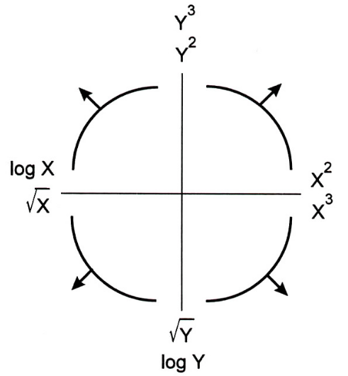
• The bottom-left quadrant appears to match the shape of the scatter plot between 'horsepower' and 'mpg' the best – let's try taking the log of 'horsepower' ($X$).

mpg['log hp'] = np.log(mpg['horsepower'])

• What does our data look like now?

px.scatter(mpg, x='log hp', y='mpg')

Predicting 'mpg' using log('horsepower')

• Let's fit another linear model.

car_model_log = LinearRegression()
car_model_log.fit(mpg[['log hp']], mpg['mpg'])

LinearRegression()

In a Jupyter environment, please rerun this cell to show the HTML representation or trust the notebook.
On GitHub, the HTML representation is unable to render, please try loading this page with nbviewer.org.

• Note that implicitly, we defined the following design matrix:

$$X = \begin{bmatrix} 1 & \log(x_1) \\ 1 & \log(x_2) \\ \vdots & \vdots \\ 1 & \log(x_n) \end{bmatrix}$$

• What do our predictions look like now?

fig = px.scatter(mpg, x='log hp', y='mpg')
log_hp_points = pd.DataFrame({'log hp': [3.7, 5.5]})
fig = px.scatter(mpg, x='log hp', y='mpg')
fig.add_trace(go.Scatter(
    x=log_hp_points['log hp'],
    y=car_model_log.predict(log_hp_points),
    mode='lines',
    name='Predicted MPG using log(Horsepower)'
))

• The fit looks a bit better! How about the $R^2$?

car_model_log.score(mpg[['log hp']], mpg['mpg'])

0.6683347641192137

• Also a bit better!

• What do our predictions look like on the original, non-transformed scatter plot? Let's see:

fig = px.scatter(mpg, x='horsepower', y='mpg')
fig.add_trace(
    go.Scatter(
        x=mpg['horsepower'], 
        y=car_model_log.intercept_ + car_model_log.coef_[0] * np.log(mpg['horsepower']),  
        mode='markers', name='Predicted MPG using log(Horsepower)'
    )
)
fig

• Our predictions that used $\log(\text{Horsepower})$ as an input don't fall on a straight line. We shouldn't expect them to; the orange dots come from:

$$\text{predicted MPG} = 108.70 - 18.582 \cdot \log(\text{Horsepower})$$

car_model_log.intercept_, car_model_log.coef_

(108.69970699574483, array([-18.58]))

Question 🤔 (Answer at practicaldsc.org/q)

Which hypothesis function is not linear in the parameters?

• A. $H(\vec{x}) = w_1 (x^{(1)} x^{(2)}) + \frac{w_2}{x^{(1)}} \sin \left( x^{(2)} \right)$
• B. $H(\vec{x}) = 2^{w_1} x^{(1)}$
• C. $H(\vec{x}) = \vec{w} \cdot \text{Aug}(\vec{x})$
• D. $H(\vec{x}) = w_1 \cos (x^{(1)}) + w_2 2^{x^{(2)} \log x^{(3)}}$
• E. More than one of the above.

What's next?

• Next class, we'll look at more examples of feature transformations.

• We'll also look at how to implement more of the feature engineering process in sklearn, ultimately creating Pipeline objects that both:
  • Define a model.
  • Define the necessary feature transformations to fit the model.