from lec_utils import *
Announcements 📣
Homework 3 is due on Thursday. See this post on Ed for an important clarification.
We've slightly adjusted the Office Hours schedule – take a look, and please come by.
I have office hours after lecture on both Tuesday and Thursday now!study.practicaldsc.org contains our discussion worksheets (and solutions), which are made up of old exam problems. Use these problems to build your theoretical understanding of the material!
Agenda
- Merging practice problem.
- Exploratory data analysis.
- Data cleaning.
- Visualization.
Question 🤔 (Answer at practicaldsc.org/q)
Remember that you can always ask questions anonymously at the link above!
Consider the DataFrames div_one (left) and coach (right), shown below.
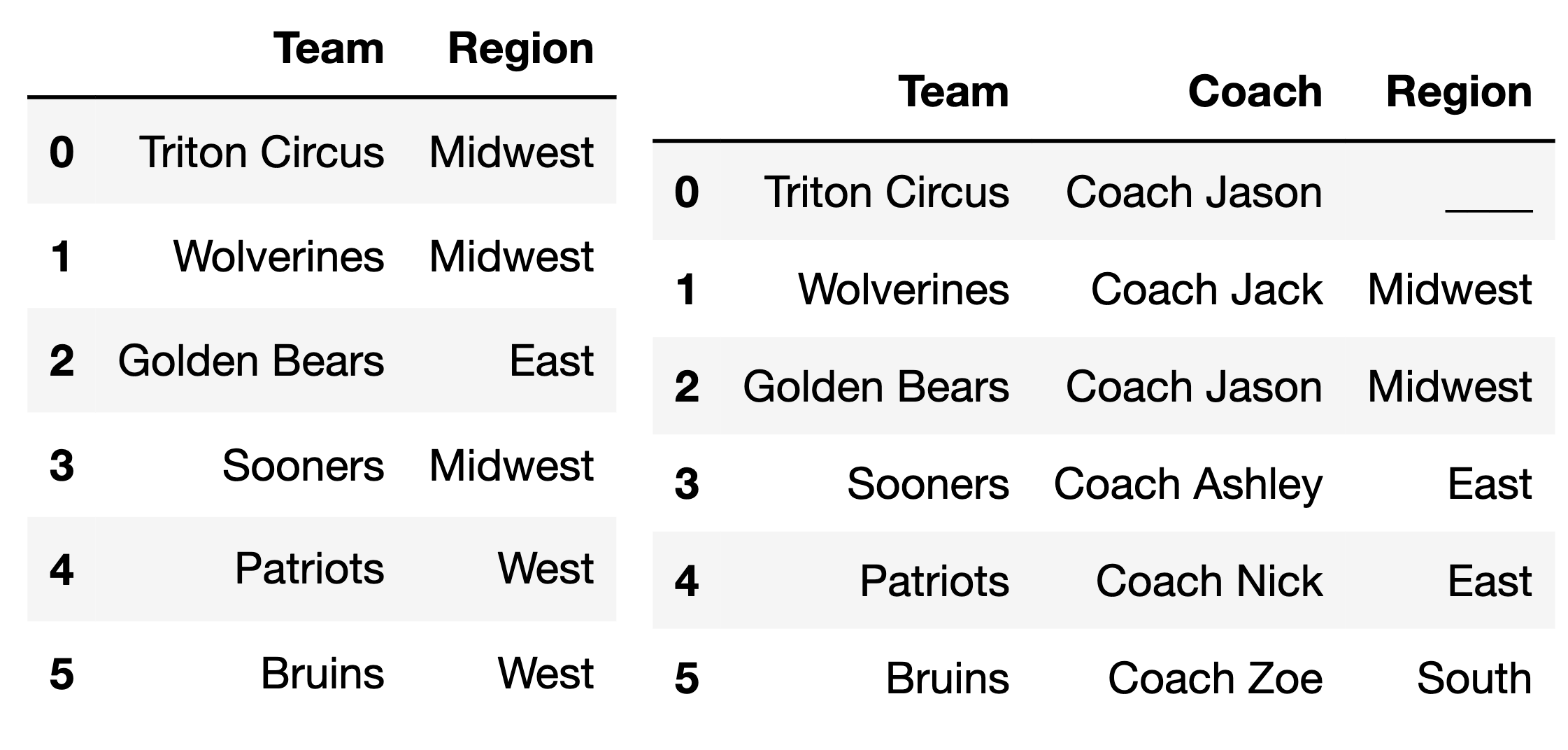
What should we fill the blank in the 'Region' column of coach so that the DataFrame div_one.merge(coach, on='Region') has 9 rows?
- A.
'South'. - B.
'West'. - C.
'East'. - D.
'Midwest'.
After you've voted, try it out yourself below.
ChatGPT doesn't even know the right answer – try asking it!
div_one = pd.DataFrame().assign(
    Team=['Triton Circus', 'Wolverines', 'Golden Bears', 'Sooners', 'Patriots', 'Bruins'],
    Region=['Midwest', 'Midwest', 'East', 'Midwest', 'West', 'West']
)
coach = pd.DataFrame().assign(
    Team=['Triton Circus', 'Wolverines', 'Golden Bears', 'Sooners', 'Patriots', 'Bruins'],
    Coach=['Coach Jason', 'Coach Jack', 'Coach Jason', 'Coach Ashley', 'Coach Nick', 'Coach Zoe'],
    Region=['____', 'Midwest', 'Midwest', 'East', 'East', 'South'] # Test this out once you've guessed!
)
# div_one.merge(coach, on='Region').shape[0]
Exploratory data analysis
Dataset overview
- LendingClub is a platform that allows individuals to borrow money – that is, take on loans.
- Each row of the dataset corresponds to a different loan that the LendingClub approved and paid out.
The full dataset is over 300 MB, so we've sampled a subset for this lecture.
loans = pd.read_csv('data/loans.csv')
# Each time you run this cell, you'll see a different random subset of the DataFrame.
loans.sample(5)
| id | loan_amnt | issue_d | term | ... | fico_range_low | fico_range_high | hardship_flag | mths_since_last_delinq | |
|---|---|---|---|---|---|---|---|---|---|
| 1345 | 120022770 | 20000.0 | Sep-2017 | 36 months | ... | 680.0 | 684.0 | N | 10.0 |
| 1659 | 129128743 | 14000.0 | Feb-2018 | 36 months | ... | 800.0 | 804.0 | N | NaN |
| 5866 | 143962984 | 15000.0 | Nov-2018 | 60 months | ... | 765.0 | 769.0 | N | NaN |
| 5828 | 145216436 | 15000.0 | Dec-2018 | 36 months | ... | 700.0 | 704.0 | N | NaN |
| 1012 | 66485750 | 10000.0 | Dec-2015 | 36 months | ... | 830.0 | 834.0 | N | NaN |
5 rows × 20 columns
# When a DataFrame has more columns than you can see in its preview,
# it's a good idea to check the names of all columns.
loans.columns
Index(['id', 'loan_amnt', 'issue_d', 'term', 'int_rate', 'grade', 'sub_grade',
       'emp_title', 'verification_status', 'home_ownership', 'annual_inc',
       'loan_status', 'purpose', 'desc', 'addr_state', 'dti', 'fico_range_low',
       'fico_range_high', 'hardship_flag', 'mths_since_last_delinq'],
      dtype='object')
- Not all of the columns are necessarily interesting, but here are some that might be:
FICO scores refer to credit scores.
# Again, run this a few times to get a sense of the typical values.
loans[['loan_amnt', 'issue_d', 'term', 'int_rate', 'emp_title', 'fico_range_low']].sample(5)
| loan_amnt | issue_d | term | int_rate | emp_title | fico_range_low | |
|---|---|---|---|---|---|---|
| 2110 | 29600.0 | Aug-2011 | 60 months | 19.69 | cbs corporation | 690.0 |
| 272 | 29725.0 | Aug-2018 | 60 months | 18.94 | account executive | 725.0 |
| 805 | 5400.0 | Oct-2017 | 36 months | 10.91 | auto body technician | 710.0 |
| 1029 | 24000.0 | Dec-2015 | 60 months | 13.67 | enterprise architect | 670.0 |
| 3886 | 17225.0 | Apr-2016 | 36 months | 16.29 | research project manager | 700.0 |
Lender decision-making
- Larger interest rates make the loan more expensive for the borrower – as a borrower, you want a lower interest rate!
- Even for the same loan amount, different borrowers were approved for different terms and interest rates:
display_df(loans.loc[loans['loan_amnt'] == 3600, ['loan_amnt', 'term', 'int_rate']], rows=17)
| loan_amnt | term | int_rate | |
|---|---|---|---|
| 249 | 3600.0 | 36 months | 24.50 |
| 626 | 3600.0 | 36 months | 13.99 |
| 1020 | 3600.0 | 36 months | 11.49 |
| 2141 | 3600.0 | 36 months | 10.08 |
| 2145 | 3600.0 | 36 months | 5.32 |
| 2584 | 3600.0 | 36 months | 16.29 |
| 2739 | 3600.0 | 36 months | 8.24 |
| 3845 | 3600.0 | 36 months | 13.66 |
| 4153 | 3600.0 | 36 months | 12.59 |
| 4368 | 3600.0 | 36 months | 14.08 |
| 4575 | 3600.0 | 36 months | 16.46 |
| 4959 | 3600.0 | 36 months | 10.75 |
| 4984 | 3600.0 | 36 months | 13.99 |
| 5478 | 3600.0 | 60 months | 10.59 |
| 5560 | 3600.0 | 36 months | 19.99 |
| 5693 | 3600.0 | 36 months | 13.99 |
| 6113 | 3600.0 | 36 months | 15.59 |
- Why do different borrowers receive different terms and interest rates?
Exploratory data analysis (EDA)
- Historically, data analysis was dominated by formal statistics, including tools like confidence intervals, hypothesis tests, and statistical modeling.
In 1977, John Tukey defined the term exploratory data analysis, which described a philosophy for proceeding about data analysis:
Exploratory data analysis is actively incisive, rather than passively descriptive, with real emphasis on the discovery of the unexpected.
Practically, EDA involves, among other things, computing summary statistics and drawing plots to understand the nature of the data at hand.
The greatest gains from data come from surprises… The unexpected is best brought to our attention by pictures.
- We'll discuss specific visualization techniques towards the end of the lecture.
Terminology
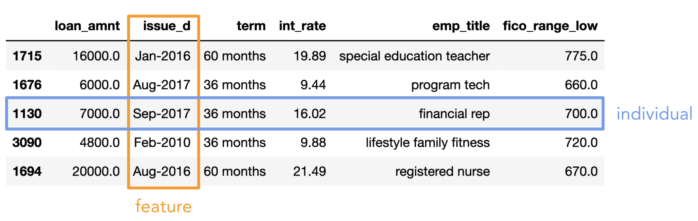
- Individual (row): Person/place/thing for which data is recorded. Also called an observation.
- Feature (column): Something that is recorded for each individual. Also called a variable or attribute.
Here, "variable" doesn't mean Python variable!
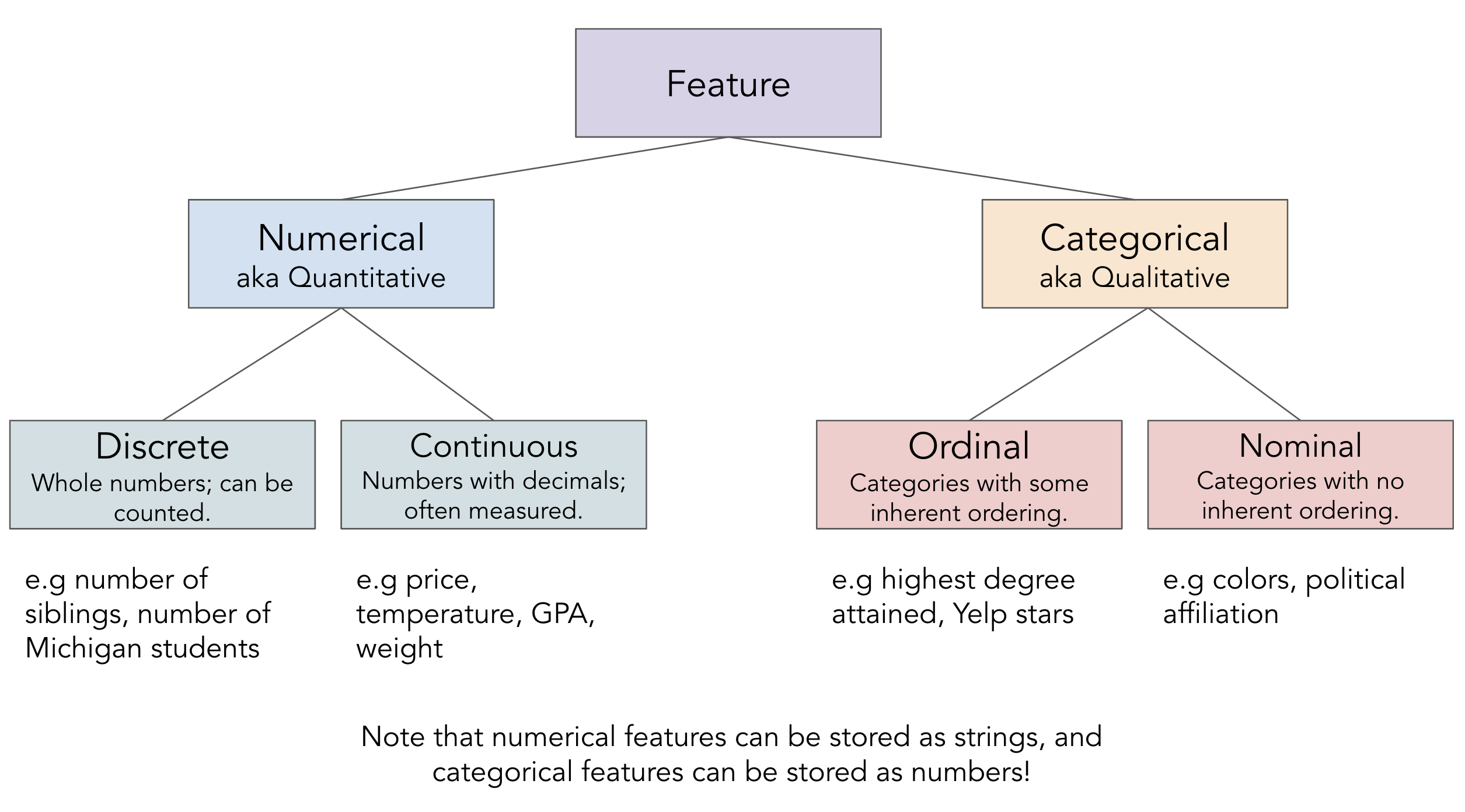
- There are two key types of features:
- Numerical features: It makes sense to do arithmetic with the values.
- Categorical features: Values fall into categories, that may or may not have some order to them.
Feature types
Question 🤔 (Answer at practicaldsc.org/q)
Remember that you can always ask questions anonymously at the link above!
Which of these are not a numerical feature?
- A. Fuel economy in miles per gallon.
- B. Zip codes.
- C. Number of semesters at Michigan.
- D. Bank account number.
- E. More than one of these are not numerical features.
Feature types vs. data types
- The data type
pandasuses is not the same as the "feature type" we talked about just now!
There's a difference between feature type (categorical, numerical) and computational data type (string, int, float, etc.).
- Be careful: sometimes numerical features are stored as strings, and categorical features are stored as numbers.
# The 'id's are stored as numbers, but are categorical (nominal).
# Are these loan 'id's (unique to each loan) or customer 'id's (which could be duplicated)?
# We'll investigate soon!
loans['id']
0        17965023
1       111414087
2        95219557
          ...
6297     63990101
6298     37641672
6299     50587446
Name: id, Length: 6300, dtype: int64
# Loan 'term's are stored as strings, but are actually numerical (discrete).
loans['term']
0        60 months
1        36 months
2        36 months
           ...
6297     60 months
6298     60 months
6299     60 months
Name: term, Length: 6300, dtype: object
Data cleaning
Four pillars of data cleaning
When loading in a dataset, to clean the data – that is, to prepare it for further analysis – we will:
- Perform data quality checks.
- Identify and handle missing values.
- Perform transformations, including converting time series data to timestamps.
- Modify structure as necessary.
Data cleaning: Data quality checks
Data quality checks
We often start an analysis by checking the quality of the data.
- Scope: Do the data match your understanding of the population?
- Measurements and values: Are the values reasonable?
- Relationships: Are related features in agreement?
- Analysis: Which features might be useful in a future analysis?
Scope: Do the data match your understanding of the population?
- Who does the data represent?
- We were told that we're only looking at approved loans. What's the distribution of
'loan_status'es?
loans.columns
Index(['id', 'loan_amnt', 'issue_d', 'term', 'int_rate', 'grade', 'sub_grade',
       'emp_title', 'verification_status', 'home_ownership', 'annual_inc',
       'loan_status', 'purpose', 'desc', 'addr_state', 'dti', 'fico_range_low',
       'fico_range_high', 'hardship_flag', 'mths_since_last_delinq'],
      dtype='object')
loans['loan_status'].value_counts()
loan_status
Fully Paid                                            3025
Current                                               2367
Charged Off                                            814
Late (31-120 days)                                      59
In Grace Period                                         23
Late (16-30 days)                                       11
Does not meet the credit policy. Status:Fully Paid       1
Name: count, dtype: int64
- Are the loans in our dataset specific to any particular state?
loans['addr_state'].value_counts().head()
addr_state
CA    905
TX    553
NY    498
FL    420
IL    261
Name: count, dtype: int64
- Were loans only given to applicants with excellent credit? Or were applicants with average credit approved for loans too?
loans['fico_range_low'].describe()
count    6300.00
mean      698.18
std        32.50
          ...
50%       690.00
75%       715.00
max       845.00
Name: fico_range_low, Length: 8, dtype: float64
Measurements and values: Are the values reasonable?
- What's the distribution of
'loan_amnt's?
Run the cell below, then read this article by the LendingClub.
# It seems like no loans were above $40,000.
loans['loan_amnt'].agg(['min', 'median', 'mean', 'max'])
min        1000.0
median    15000.0
mean      15568.8
max       40000.0
Name: loan_amnt, dtype: float64
- What kinds of information does the
loansDataFrame even hold?
# The "object" dtype in pandas refers to anything that is not numeric/Boolean/time-related,
# including strings.
loans.info()
<class 'pandas.core.frame.DataFrame'>
RangeIndex: 6300 entries, 0 to 6299
Data columns (total 20 columns):
 #   Column                  Non-Null Count  Dtype
---  ------                  --------------  -----
 0   id                      6300 non-null   int64
 1   loan_amnt               6300 non-null   float64
 2   issue_d                 6300 non-null   object
 3   term                    6300 non-null   object
 4   int_rate                6300 non-null   float64
 5   grade                   6300 non-null   object
 6   sub_grade               6300 non-null   object
 7   emp_title               6300 non-null   object
 8   verification_status     6300 non-null   object
 9   home_ownership          6300 non-null   object
 10  annual_inc              6300 non-null   float64
 11  loan_status             6300 non-null   object
 12  purpose                 6300 non-null   object
 13  desc                    324 non-null    object
 14  addr_state              6300 non-null   object
 15  dti                     6299 non-null   float64
 16  fico_range_low          6300 non-null   float64
 17  fico_range_high         6300 non-null   float64
 18  hardship_flag           6300 non-null   object
 19  mths_since_last_delinq  3120 non-null   float64
dtypes: float64(7), int64(1), object(12)
memory usage: 984.5+ KB
- What's going on in the
'id'column ofrest?
# Are there multiple rows with the same 'id'?
# That is, are they person 'id's or loan 'id's?
loans['id'].value_counts().max()
1
Relationships: Are related features in agreement?
- Why are there two columns with credit scores,
'fico_range_low'and'fico_range_high'? What do they both mean?
loans[['fico_range_low', 'fico_range_high']]
| fico_range_low | fico_range_high | |
|---|---|---|
| 0 | 700.0 | 704.0 |
| 1 | 680.0 | 684.0 |
| 2 | 705.0 | 709.0 |
| ... | ... | ... |
| 6297 | 675.0 | 679.0 |
| 6298 | 660.0 | 664.0 |
| 6299 | 685.0 | 689.0 |
6300 rows × 2 columns
(loans['fico_range_high'] - loans['fico_range_low']).value_counts()
4.0    6298
5.0       2
Name: count, dtype: int64
- Does every
'sub_grade'align with its related'grade'?
loans[['grade', 'sub_grade']]
| grade | sub_grade | |
|---|---|---|
| 0 | D | D3 |
| 1 | C | C5 |
| 2 | A | A5 |
| ... | ... | ... |
| 6297 | E | E2 |
| 6298 | C | C4 |
| 6299 | B | B3 |
6300 rows × 2 columns
# Turns out, the answer is yes!
# The .str accessor allows us to use the [0] operation
# on every string in loans['sub_grade'].
(loans['sub_grade'].str[0] == loans['grade']).all()
True
Data cleaning: Missing values
Missing values
- Next, it's important to check for and handle missing value, i.e. null values, as they can have a big effect on your analysis.
# Note that very few of the 'desc' (description) values are non-null!
loans.info()
<class 'pandas.core.frame.DataFrame'>
RangeIndex: 6300 entries, 0 to 6299
Data columns (total 20 columns):
 #   Column                  Non-Null Count  Dtype
---  ------                  --------------  -----
 0   id                      6300 non-null   int64
 1   loan_amnt               6300 non-null   float64
 2   issue_d                 6300 non-null   object
 3   term                    6300 non-null   object
 4   int_rate                6300 non-null   float64
 5   grade                   6300 non-null   object
 6   sub_grade               6300 non-null   object
 7   emp_title               6300 non-null   object
 8   verification_status     6300 non-null   object
 9   home_ownership          6300 non-null   object
 10  annual_inc              6300 non-null   float64
 11  loan_status             6300 non-null   object
 12  purpose                 6300 non-null   object
 13  desc                    324 non-null    object
 14  addr_state              6300 non-null   object
 15  dti                     6299 non-null   float64
 16  fico_range_low          6300 non-null   float64
 17  fico_range_high         6300 non-null   float64
 18  hardship_flag           6300 non-null   object
 19  mths_since_last_delinq  3120 non-null   float64
dtypes: float64(7), int64(1), object(12)
memory usage: 984.5+ KB
# Run this repeatedly to read a random sample of loan descriptions.
for desc in loans.loc[loans['desc'].notna(), 'desc'].sample(3):
    print(desc + '\n')
  Borrower added on 04/24/13 > To pay off credit card debt.<br>

  Borrower added on 04/19/13 > Have three credit cards that have teaser rates of zero percent APR's that are about to expire.<br>

  Borrower added on 05/16/13 > for credit cards and personal things<br><br> Borrower added on 05/16/13 > I need it for my credit cards and personal items<br><br> Borrower added on 05/16/13 > I need it for my credit cards and would like to use it for things that I would like to get.<br><br> Borrower added on 05/16/13 > I would like it for credit cards and personal things I would like to get for myself.  I work hard and think it would be nice to get a few things I would like to get at one time instead of waiting until I can save enough money that never seems to work.  I save a little but not alot in good time......<br>
- The
.isna()Series method checks whether each element in a Series is missing (True) or present (False)..notna()does the opposite.
# The percentage of values in each column that are missing.
loans.isna().mean().sort_values(ascending=False) * 100
desc                      94.86
mths_since_last_delinq    50.48
dti                        0.02
                          ...
term                       0.00
issue_d                    0.00
annual_inc                 0.00
Length: 20, dtype: float64
- It appears that applicants who submitted descriptions with their loan applications were given higher interest rates on average than those who didn't submit descriptions.
But, this could've happened for a variety of reasons, not just because they submitted a description.
(
    loans
    .assign(submitted_description=loans['desc'].notna())
    .groupby('submitted_description')
    ['int_rate']
    .agg(['mean', 'median'])
)
| mean | median | |
|---|---|---|
| submitted_description | ||
| False | 13.09 | 12.62 |
| True | 13.68 | 13.68 |
- There are many ways of handling missing values, which we'll discuss more in a future lecture. But a good first step is to check how many there are!
Aside: Series operations with null values
- The
numpy/pandasnull value,np.nan, is typically ignored when usingnumpy/pandasoperations.
# Note the NaN at the very bottom.
loans['mths_since_last_delinq']
0       72.0
1        6.0
2       66.0
        ...
6297    39.0
6298    22.0
6299     NaN
Name: mths_since_last_delinq, Length: 6300, dtype: float64
loans['mths_since_last_delinq'].sum()
106428.0
- But,
np.nans typically aren't ignored when using regular Python operations.
sum(loans['mths_since_last_delinq'])
nan
- As an aside, the regular Python null value is
None.
None
np.nan
nan
Data cleaning: Transformations and timestamps
Transformations
- A transformation results from performing some operation on every element in a sequence, e.g. a Series.
- When preparing data for analysis, we often need to:
- Perform type conversions (e.g. changing the string
'$2.99'to the float2.99). - Perform unit conversions (e.g. feet to meters).
- Extract relevant information from strings.
- Perform type conversions (e.g. changing the string
- For example, we can't currently use the
'term'column to do any calculations, since its values are stored as strings (despite being numerical).
loans['term']
0        60 months
1        36 months
2        36 months
           ...
6297     60 months
6298     60 months
6299     60 months
Name: term, Length: 6300, dtype: object
- Many of the values in
'emp_title'are stored inconsistently, meaning they mean the same thing, but appear differently. Without further cleaning, this would make it harder to, for example, find the total number of nurses that were given loans.
(loans['emp_title'] == 'registered nurse').sum()
252
(loans['emp_title'] == 'nurse').sum()
101
(loans['emp_title'] == 'rn').sum()
35
One solution: The apply method
- The Series
applymethod allows us to use a function on every element in a Series.
def clean_term(term_string):
    return int(term_string.split()[0])
loans['term'].apply(clean_term)
0       60
1       36
2       36
        ..
6297    60
6298    60
6299    60
Name: term, Length: 6300, dtype: int64
- There is also an
applymethod for DataFrames, in which you can use a function on every row (if you setaxis=1) or every column (if you setaxis=0) of a DataFrame.
- There is also an
applymethod for DataFrameGroupBy/SeriesGroupBy objects, as you're seeing in Question 2.3 of Homework 3!
The price of apply
- Unfortunately,
applyruns really slowly!
%%timeit
loans['term'].apply(clean_term)
1.67 ms ± 81.2 μs per loop (mean ± std. dev. of 7 runs, 1,000 loops each)
%%timeit
res = []
for term in loans['term']:
    res.append(clean_term(term))
1.36 ms ± 17.6 μs per loop (mean ± std. dev. of 7 runs, 1,000 loops each)
- Internally,
applyactually just runs afor-loop!
- So, when possible – say, when applying arithmetic operations – we should work on Series objects directly and avoid
apply!
%%timeit
loans['int_rate'] // 10 * 10 # Rounds down to the nearest multiple of 10.
89.8 μs ± 803 ns per loop (mean ± std. dev. of 7 runs, 10,000 loops each)
%%timeit
loans['int_rate'].apply(lambda y: y // 10 * 10)
716 μs ± 6.95 μs per loop (mean ± std. dev. of 7 runs, 1,000 loops each)
- Above, the solution involving
applyis ~10x slower than the one that uses direct vectorized operations.
The .str accessor
- For string operations,
pandasprovides a convenient.straccessor.
You've seen examples of it in practice already, with.str.contains, and also with.str[0]earlier in today's lecture.
- Mental model: the operations that come after
.strare used on every single element of the Series that comes before.str.
# Here, we use .split() on every string in loans['term'].
loans['term'].str.split()
0       [60, months]
1       [36, months]
2       [36, months]
            ...
6297    [60, months]
6298    [60, months]
6299    [60, months]
Name: term, Length: 6300, dtype: object
loans['term'].str.split().str[0].astype(int)
0       60
1       36
2       36
        ..
6297    60
6298    60
6299    60
Name: term, Length: 6300, dtype: int64
- One might think that it's quicker than
apply, but it's actually even slower. But, we still use it in practice since it allows us to write concise code.
Creating timestamps ⏱️
- When dealing with values containing dates and times, it's good practice to convert the values to "timestamp" objects.
# Stored as strings.
loans['issue_d']
0       Jun-2014
1       Jun-2017
2       Dec-2016
          ...
6297    Nov-2015
6298    Dec-2014
6299    Jun-2015
Name: issue_d, Length: 6300, dtype: object
- To do so, we use the
pd.to_datetimefunction.
It takes in a date format string; you can see examples of how they work here.
pd.to_datetime(loans['issue_d'], format='%b-%Y')
0      2014-06-01
1      2017-06-01
2      2016-12-01
          ...
6297   2015-11-01
6298   2014-12-01
6299   2015-06-01
Name: issue_d, Length: 6300, dtype: datetime64[ns]
Aside: The pipe method🚰
- There are a few steps we've performed to clean up our dataset.
- Convert loan
'term's to integers. - Convert loan issue dates,
'issue_d's, to timestamps.
- Convert loan
- When we manipulate DataFrames, it's best to define individual functions for each step, then use the
pipemethod to chain them all together.
Thepipemethod takes in a function, which itself takes in DataFrame and returns a DataFrame.
def clean_term_column(df):
    return df.assign(
        term=df['term'].str.split().str[0].astype(int)
    )
def clean_date_column(df):
    return (
        df
        .assign(date=pd.to_datetime(df['issue_d'], format='%b-%Y'))
        .drop(columns=['issue_d'])
    )
loans = (
    pd.read_csv('data/loans.csv')
    .pipe(clean_term_column)
    .pipe(clean_date_column)
)
loans
| id | loan_amnt | term | int_rate | ... | fico_range_high | hardship_flag | mths_since_last_delinq | date | |
|---|---|---|---|---|---|---|---|---|---|
| 0 | 17965023 | 18000.0 | 60 | 16.99 | ... | 704.0 | N | 72.0 | 2014-06-01 |
| 1 | 111414087 | 10000.0 | 36 | 16.02 | ... | 684.0 | N | 6.0 | 2017-06-01 |
| 2 | 95219557 | 12800.0 | 36 | 7.99 | ... | 709.0 | N | 66.0 | 2016-12-01 |
| ... | ... | ... | ... | ... | ... | ... | ... | ... | ... |
| 6297 | 63990101 | 10800.0 | 60 | 18.49 | ... | 679.0 | N | 39.0 | 2015-11-01 |
| 6298 | 37641672 | 15000.0 | 60 | 14.31 | ... | 664.0 | N | 22.0 | 2014-12-01 |
| 6299 | 50587446 | 14000.0 | 60 | 9.99 | ... | 689.0 | N | NaN | 2015-06-01 |
6300 rows × 20 columns
# Same as above, just way harder to read and write.
clean_date_column(clean_term_column(pd.read_csv('data/loans.csv')))
| id | loan_amnt | term | int_rate | ... | fico_range_high | hardship_flag | mths_since_last_delinq | date | |
|---|---|---|---|---|---|---|---|---|---|
| 0 | 17965023 | 18000.0 | 60 | 16.99 | ... | 704.0 | N | 72.0 | 2014-06-01 |
| 1 | 111414087 | 10000.0 | 36 | 16.02 | ... | 684.0 | N | 6.0 | 2017-06-01 |
| 2 | 95219557 | 12800.0 | 36 | 7.99 | ... | 709.0 | N | 66.0 | 2016-12-01 |
| ... | ... | ... | ... | ... | ... | ... | ... | ... | ... |
| 6297 | 63990101 | 10800.0 | 60 | 18.49 | ... | 679.0 | N | 39.0 | 2015-11-01 |
| 6298 | 37641672 | 15000.0 | 60 | 14.31 | ... | 664.0 | N | 22.0 | 2014-12-01 |
| 6299 | 50587446 | 14000.0 | 60 | 9.99 | ... | 689.0 | N | NaN | 2015-06-01 |
6300 rows × 20 columns
Working with timestamps
- We often want to adjust the granularity of timestamps to see overall trends, or seasonality.
- To do so, use the
resampleDataFrame method (documentation).
Think of it like a version ofgroupby, but for timestamps.
# This shows us the average interest rate given out to loans in every 6 month interval.
loans.resample('6M', on='date')['int_rate'].mean()
date
2008-03-31    10.71
2008-09-30     8.63
2009-03-31    12.13
              ...
2018-03-31    12.85
2018-09-30    12.72
2019-03-31    12.93
Freq: 6M, Name: int_rate, Length: 23, dtype: float64
- We can also do arithmetic with timestamps.
# Not meaningful in this example, but possible.
loans['date'].diff()
0            NaT
1      1096 days
2      -182 days
          ...
6297   -517 days
6298   -335 days
6299    182 days
Name: date, Length: 6300, dtype: timedelta64[ns]
# If each loan was for 60 months,
# this is a Series of when they'd end.
# Unfortunately, pd.DateOffset isn't vectorized, so
# if you'd want to use a different month offset for each row
# (like we'd need to, since some loans are 36 months
# and some are 60 months), you'd need to use `.apply`.
loans['date'] + pd.DateOffset(months=60)
0      2019-06-01
1      2022-06-01
2      2021-12-01
          ...
6297   2020-11-01
6298   2019-12-01
6299   2020-06-01
Name: date, Length: 6300, dtype: datetime64[ns]
The .dt accessor
- Like with Series of strings,
pandashas a.dtaccessor for properties of timestamps (documentation).
loans['date'].dt.year
0       2014
1       2017
2       2016
        ...
6297    2015
6298    2014
6299    2015
Name: date, Length: 6300, dtype: int32
loans['date'].dt.month
0        6
1        6
2       12
        ..
6297    11
6298    12
6299     6
Name: date, Length: 6300, dtype: int32
Reshaping DataFrames
We often reshape the DataFrame's structure to make it more convenient for analysis. For example, we can:
- Simplify structure by removing columns or taking a set of rows for a particular period of time or geographic area.
We already did this!
- Adjust granularity by aggregating rows together.
To do this, usegroupby(orresample, if working with timestamps).
- Reshape structure, most commonly by using the DataFrame
meltmethod to un-pivot a dataframe.
Using melt
- The
meltmethod is common enough that we'll give it a special mention.
- We'll often encounter pivot tables (esp. from government data), which we call wide data.
- The methods we've introduced work better with long-form data, or tidy data.
- To go from wide to long,
melt.

Example usage of melt
wide_example = pd.DataFrame({
    'Year': [2001, 2002],
    'Jan': [10, 130],
    'Feb': [20, 200],
    'Mar': [30, 340]
}).set_index('Year')
wide_example
| Jan | Feb | Mar | |
|---|---|---|---|
| Year | |||
| 2001 | 10 | 20 | 30 |
| 2002 | 130 | 200 | 340 |
wide_example.melt(ignore_index=False)
| variable | value | |
|---|---|---|
| Year | ||
| 2001 | Jan | 10 |
| 2002 | Jan | 130 |
| 2001 | Feb | 20 |
| 2002 | Feb | 200 |
| 2001 | Mar | 30 |
| 2002 | Mar | 340 |
Visualization
Why visualize?
- Computers are better than humans at crunching numbers, but humans are better at identifying visual patterns.
- Visualizations allow us to understand lots of data quickly – they make it easier to spot trends and communicate our results with others.
- There are many types of visualizations; the right choice depends on the type of data at hand.
In this class, we'll look at scatter plots, line plots, bar charts, histograms, choropleths, and boxplots.
Choosing the correct type of visualization
- The type of visualization we create depends on the types of features we're visualizing.
- We'll directly learn how to produce the bolded visualizations below, but the others are also options.
See more examples here.
| Feature types | Options |
|---|---|
| Single categorical feature | Bar charts, pie charts, dot plots |
| Single numerical feature | Histograms, box plots, density curves, rug plots, violin plots |
| Two numerical features | Scatter plots, line plots, heat maps, contour plots |
| One categorical and one numerical feature It really depends on the nature of the features themselves! |
Side-by-side histograms, box plots, or bar charts, overlaid line plots or density curves |
- Note that we use the words "plot", "chart", and "graph" mean the same thing.
plotly
- We've used
plotlyin lecture briefly, and you've even used it in Homework 1 and Homework 3, but we've never formally discussed it.
- It's a visualization library that enables interactive visualizations.

Using plotly
- We can use
plotlyusing theplotly.expresssyntax.plotlyis very flexible, but it can be verbose;plotly.expressallows us to make plots quickly.- See the documentation here – it's very rich.
There are good examples for almost everything!
import plotly.express as px
- Alternatively, we can use
plotlyby settingpandasplotting backend to'plotly'and using the DataFrame/Seriesplotmethod.
By default, the plotting backend ismatplotlib, which creates non-interactive visualizations.
pd.options.plotting.backend = 'plotly'
- Now, we're going to look at several examples. Focus on what is being visualized and why; read the notebook later for the how.
Bar charts
- Bar charts are used to show:
- The distribution of a single categorical feature, or
- The relationship between one categorical feature and one numerical feature.
- Usage:
px.bar/px.barhordf.plot(kind='bar)'/df.plot(kind='barh').'h'stands for "horizontal."
- Example: What is the distribution of
'addr_state's inloans?
# Here, we're using the .plot method on loans['addr_state'], which is a Series.
# We prefer horizontal bar charts, since they're easier to read.
(
    loans['addr_state']
    .value_counts()
    .plot(kind='barh')
)
# A little formatting goes a long way!
(
    loans['addr_state']
    .value_counts()
    .sort_values()
    .head(10)
    .plot(kind='barh', title='States of Residence for Successful Loan Applicants')
    .update_layout()
)
- Example: What is the average
'int_rate'for each'home_ownership'status?
(
    loans
    .groupby('home_ownership')
    ['int_rate']
    .mean()
    .plot(kind='barh', title='Average Interest Rate by Home Ownership Status')
)
# The "ANY" category seems to be an outlier.
loans['home_ownership'].value_counts()
home_ownership
MORTGAGE    2810
RENT        2539
OWN          950
ANY            1
Name: count, dtype: int64
Side-by-side bar charts
- Instead of just looking at
'int_rate's for different,'home_ownership'statuses, we could also group by loan'term's, too. As we'll see,'term'impacts'int_rate'far more than'home_ownership'.
(
    loans
    .groupby('home_ownership')
    .filter(lambda df: df.shape[0] > 1) # Gets rid of the "ANY" category.
    .groupby(['home_ownership', 'term'])
    [['int_rate']]
    .mean()
)
| int_rate | ||
|---|---|---|
| home_ownership | term | |
| MORTGAGE | 36 | 11.42 |
| 60 | 15.27 | |
| OWN | 36 | 11.75 |
| 60 | 16.14 | |
| RENT | 36 | 12.23 |
| 60 | 16.43 |
- A side-by-side bar chart, which we can create by setting the
colorandbarmodearguments, makes the pattern clear:
# Annoyingly, the side-by-side bar chart doesn't work properly
# if the column that separates colors (here, 'term')
# isn't made up of strings.
(
    loans
    .assign(term=loans['term'].astype(str) + ' months')
    .groupby('home_ownership')
    .filter(lambda df: df.shape[0] > 1)
    .groupby(['home_ownership', 'term'])
    [['int_rate']]
    .mean()
    .reset_index()
    .plot(kind='bar',
          y='int_rate',
          x='home_ownership',
          color='term',
          barmode='group',
          title='Average Interest Rate by Home Ownership Status and Loan Term',
          width=800)
)
- Why do longer loans have higher
'int_rate's on average?
Histograms
- The previous slide showed the average
'int_rate'for different combinations of'home_ownership'status and'term'. But what if we want to visualize more about'int_rate's than just their average?
- Histograms are used to show the distribution of a single numerical feature.
- Usage:
px.histogramordf.plot(kind='hist').
- Example: What is the distribution of
'int_rate'?
(
    loans
    .plot(kind='hist', x='int_rate', title='Distribution of Interest Rates')
)
- With fewer bins, we see less detail (and less noise) in the shape of the distribution.
Play with the slider that appears when you run the cell below!
from ipywidgets import interact
def hist_bins(nbins):
    (
        loans
        .plot(kind='hist', x='int_rate', nbins=nbins, title='Distribution of Interest Rates')
        .show()
    )
interact(hist_bins, nbins=(1, 51));
interactive(children=(IntSlider(value=26, description='nbins', max=51, min=1), Output()), _dom_classes=('widge…
Box plots and violin plots
- Box plots and violin plots are alternatives to histograms, in that they also are used to show the distribution of quantitative features.
Learn more about box plots here.
- The benefit to them is that they're easily stacked side-by-side to compare distributions.
- Example: What is the distribution of
'int_rate'?
(
    loans
    .plot(kind='hist', x='int_rate', title='Distribution of Interest Rates')
)
- Example: What is the distribution of
'int_rate', separately for each loan'term'?
(
    loans
    .plot(kind='box', y='int_rate', color='term', orientation='v',
          title='Distribution of Interest Rates by Loan Term')
)
(
    loans
    .plot(kind='violin', y='int_rate', color='term', orientation='v',
          title='Distribution of Interest Rates by Loan Term')
)
- Overlaid histograms can be used to show the distributions of multiple numerical features, too.
(
    loans
    .plot(kind='hist', x='int_rate', color='term', marginal='box', nbins=20,
          title='Distribution of Interest Rates by Loan Term')
)
Scatter plots
- Scatter plots are used to show the relationship between two quantitative features.
- Usage:
px.scatterordf.plot(kind='scatter').
- Example: What is the relationship between
'int_rate'and debt-to-income ratio,'dti'?
(
    loans
    .sample(200, random_state=23)
    .plot(kind='scatter', x='dti', y='int_rate', title='Interest Rate vs. Debt-to-Income Ratio')
)
- There are a multitude of ways that scatter plots can be customized. We can color points based on groups, we can resize points based on another numeric column, we can give them hover labels, etc.
(
    loans
    .assign(term=loans['term'].astype(str))
    .sample(200, random_state=23)
    .plot(kind='scatter', x='dti', y='int_rate', color='term',
          hover_name='id', size='loan_amnt',
          title='Interest Rate vs. Debt-to-Income Ratio')
)
Line charts
- Line charts are used to show how one quantitative feature changes over time.
- Usage:
px.lineordf.plot(kind='line').
- Example: How many loans were given out each year in our dataset?
This is likely not true of the market in general, or even LendingClub in general, but just a consequence of where our dataset came from.
(
    loans
    .assign(year=loans['date'].dt.year)
    ['year']
    .value_counts()
    .sort_index()
    .plot(kind='line', title='Number of Loans Given Per Year')
)
- Example: How has the average
'int_rate'changed over time?
(
    loans
    .resample('6M', on='date')
    ['int_rate']
    .mean()
    .plot(kind='line', title='Average Interest Rate over Time')
)
- Example: How has the average
'int_rate'changed over time, separately for 36 month and 60 month loans?
(
    loans
    .groupby('term')
    .resample('6M', on='date')
    ['int_rate']
    .mean()
    .reset_index()
    .plot(kind='line', x='date', y='int_rate', color='term',
          title='Average Interest Rate over Time')
)