from lec_utils import *
def show_grouping_animation():
    src = "https://docs.google.com/presentation/d/1tBaFyHseIGsX5wmE3BdNLeVHnKksQtpzLhHge8Tzly0/embed?start=false&loop=false&delayms=60000&rm=minimal"
    width = 960
    height = 509
    display(IFrame(src, width, height))
def show_merging_animation():
    src = "https://docs.google.com/presentation/d/1HPJ7fiBLNEURsWYiY0qpqPR3qup68Mr0_B34GU99Y8Q/embed?start=false&loop=false&delayms=60000&rm=minimal"
    width = 865
    height = 509
    display(IFrame(src, width, height))
Announcements 📣
- Homework 2 is due tomorrow night – we've provided a 24-hour extension to everyone since we released it a bit late. Don't be discouraged if you feel like there's a lot of reading or you have to do a lot of Googling – this is intentional, because this is how data scientists actually have to solve problems!
Post on Ed or
come to Office Hours for help! We're using a queue for office hours now – access it from practicaldsc.org/calendar.
study.practicaldsc.org contains our discussion worksheets (and solutions), which are made up of old exam problems. Use these problems to build your theoretical understanding of the material!
Homework 1 scores are available on Gradescope.
Now, you can even see which hidden tests you failed.
Agenda
- Recap:
groupby. - Advanced
groupbyusage. - Pivot tables using the
pivot_tablemethod. - Merging.
Remember to follow along in lecture by accessing the "blank" lecture notebook in our public GitHub repository.
Question 🤔 (Answer at practicaldsc.org/q)
Remember that you can always ask questions anonymously at the link above!
We have 2 office hours on Central Campus each week, but not many students have attended. What should we do with them?
- A. Keep them – I'll come at some point.
- B. Keep them on Central Campus, but change them to a different time (let us know when in the free response box).
- C. Replace them with more North Campus Office hours (let us know when in the free response box).
show_grouping_animation()
Run the cell below to load in our dataset.
penguins = sns.load_dataset('penguins').dropna().reset_index(drop=True)
penguins
| species | island | bill_length_mm | bill_depth_mm | flipper_length_mm | body_mass_g | sex | |
|---|---|---|---|---|---|---|---|
| 0 | Adelie | Torgersen | 39.1 | 18.7 | 181.0 | 3750.0 | Male |
| 1 | Adelie | Torgersen | 39.5 | 17.4 | 186.0 | 3800.0 | Female |
| 2 | Adelie | Torgersen | 40.3 | 18.0 | 195.0 | 3250.0 | Female |
| ... | ... | ... | ... | ... | ... | ... | ... |
| 330 | Gentoo | Biscoe | 50.4 | 15.7 | 222.0 | 5750.0 | Male |
| 331 | Gentoo | Biscoe | 45.2 | 14.8 | 212.0 | 5200.0 | Female |
| 332 | Gentoo | Biscoe | 49.9 | 16.1 | 213.0 | 5400.0 | Male |
333 rows × 7 columns
Example: Finding the mean 'bill_length_mm' of each species
- If you were asked to find the mean
'bill_length_mm'of'Adelie'penguins, you could do so using a query.
penguins.loc[penguins['species'] == 'Adelie', 'bill_length_mm'].mean()
38.82397260273973
- But, you can find the mean
'bill_length_mm'of all three species usinggroupby:
# Read this as:
#        for each 'species',  calculate the mean 'bill_length_mm'.
penguins.groupby('species')['bill_length_mm'].mean()
species
Adelie       38.82
Chinstrap    48.83
Gentoo       47.57
Name: bill_length_mm, dtype: float64
Understanding the syntax of groupby
penguins.groupby('species')['bill_length_mm'].mean()
First, tellpandaswhich column you want to group by. Since we're grouping by'species', the remainder of the calculations will be done separately for each'species'.
penguins.groupby('species')['bill_length_mm'].mean()
Then, select the other column(s) that you want to aggregate. Here, we want to calculate mean'bill_length_m's, so that's what we select.
penguins.groupby('species')['bill_length_mm'].mean()
Finally, we use an aggregation method. This is saying, for each'species', compute the mean'bill_length_mm'.
Advanced groupby usage
Beyond default aggregation methods
- There are many built-in aggregation methods.
- What if you want to apply different aggregation methods to different columns?
- What if the aggregation method you want to use doesn't already exist in
pandas?
The aggregate method
DataFrameGroupByandSeriesGroupByobjects have a generalaggregatemethod, which aggregates using one or more operations.
Remember, aggregation is the act of combining many values into a single value.
- There are many ways of using
aggregate; refer to the documentation for a comprehensive list.
Per the documentation,aggis an alias foraggregate.
- Example arguments:
- A single function.
- A list of functions.
- A dictionary mapping column names to functions.
- We've attached a Reference Slide with examples.
- How many penguins are there of each
'species', and what is the mean'body_mass_g'of each'species'?
(
    penguins
    .groupby('species')
    ['body_mass_g']
    .aggregate(['count', 'mean'])
)
| count | mean | |
|---|---|---|
| species | ||
| Adelie | 146 | 3706.16 |
| Chinstrap | 68 | 3733.09 |
| Gentoo | 119 | 5092.44 |
- What is the maximum
'bill_length_mm'of each'species', and which'island's is each'species'found on?
(
    penguins
    .groupby('species')
    .agg({'bill_length_mm': 'max', 'island': 'unique'})
)
| bill_length_mm | island | |
|---|---|---|
| species | ||
| Adelie | 46.0 | [Torgersen, Biscoe, Dream] |
| Chinstrap | 58.0 | [Dream] |
| Gentoo | 59.6 | [Biscoe] |
Activity
What is the interquartile range of the 'body_mass_g' of each 'species'?
The interquartile range of a distribution is defined as:
$$\text{75th percentile} - \text{25th percentile}$$*Hint*: Use np.percentile, and pass agg/aggregate a custom function.
# Here, the argument to agg is a function,
# which takes in a Series and returns a scalar.
def iqr(s):
    return np.percentile(s, 75) - np.percentile(s, 25)
(
    penguins
    .groupby('species')
    ['body_mass_g']
    .agg(iqr)
)
species
Adelie       637.5
Chinstrap    462.5
Gentoo       800.0
Name: body_mass_g, dtype: float64
Question 🤔 (Answer at practicaldsc.org/q)
Remember that you can always ask questions anonymously at the link above!
What questions do you have?
Split-apply-combine, revisited
- When we introduced the split-apply-combine pattern, the "apply" step involved aggregation – our final DataFrame had one row for each group.
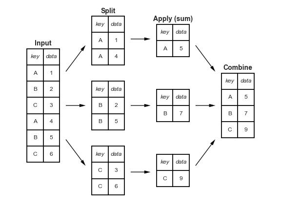
- Instead of aggregating during the apply step, we could instead perform a filtration, in which we keep only the groups that satisfy some condition.
- Or a transformation, in which we perform operations to every value within each group.
Grouping, then filtering
- To keep only the groups that satisfy a particular condition, use the
filtermethod on aDataFrameGroupBy/SeriesGroupByobject.
Thefiltermethod takes in a function, which itself takes in a DataFrame/Series and return a single Boolean. The result is a new DataFrame/Series with only the groups for which the filter function returnedTrue.
- For example, suppose we want only the
'species'whose average'bill_length_mm'is above 39.
(
    penguins
    .groupby('species')
    .filter(lambda df: df['bill_length_mm'].mean() > 39)
)
| species | island | bill_length_mm | bill_depth_mm | flipper_length_mm | body_mass_g | sex | |
|---|---|---|---|---|---|---|---|
| 146 | Chinstrap | Dream | 46.5 | 17.9 | 192.0 | 3500.0 | Female |
| 147 | Chinstrap | Dream | 50.0 | 19.5 | 196.0 | 3900.0 | Male |
| 148 | Chinstrap | Dream | 51.3 | 19.2 | 193.0 | 3650.0 | Male |
| ... | ... | ... | ... | ... | ... | ... | ... |
| 330 | Gentoo | Biscoe | 50.4 | 15.7 | 222.0 | 5750.0 | Male |
| 331 | Gentoo | Biscoe | 45.2 | 14.8 | 212.0 | 5200.0 | Female |
| 332 | Gentoo | Biscoe | 49.9 | 16.1 | 213.0 | 5400.0 | Male |
187 rows × 7 columns
- No more
'Adelie's!
Activity
Create a new DataFrame with only the rows in penguins for popular 'species' – that is, 'species' with at least 100 penguins.
(
    penguins
    .groupby('species')
    .filter(lambda df: df.shape[0] >= 100)
)
| species | island | bill_length_mm | bill_depth_mm | flipper_length_mm | body_mass_g | sex | |
|---|---|---|---|---|---|---|---|
| 0 | Adelie | Torgersen | 39.1 | 18.7 | 181.0 | 3750.0 | Male |
| 1 | Adelie | Torgersen | 39.5 | 17.4 | 186.0 | 3800.0 | Female |
| 2 | Adelie | Torgersen | 40.3 | 18.0 | 195.0 | 3250.0 | Female |
| ... | ... | ... | ... | ... | ... | ... | ... |
| 330 | Gentoo | Biscoe | 50.4 | 15.7 | 222.0 | 5750.0 | Male |
| 331 | Gentoo | Biscoe | 45.2 | 14.8 | 212.0 | 5200.0 | Female |
| 332 | Gentoo | Biscoe | 49.9 | 16.1 | 213.0 | 5400.0 | Male |
265 rows × 7 columns
# Note that to just find the 'species' with at least 100 penguins,
# we didn't need to group:
penguins['species'].value_counts()
species
Adelie       146
Gentoo       119
Chinstrap     68
Name: count, dtype: int64
- Suppose we want to convert the
'body_mass_g'column to to z-scores (i.e. standard units):
def z_score(x):
    return (x - x.mean()) / x.std(ddof=0)
z_score(penguins['body_mass_g'])
0     -0.57
1     -0.51
2     -1.19
       ...
330    1.92
331    1.23
332    1.48
Name: body_mass_g, Length: 333, dtype: float64
- Now, what if we wanted the z-score within each group?
- To do so, we can use the
transformmethod on aDataFrameGroupByobject. Thetransformmethod takes in a function, which itself takes in a Series and returns a new Series.
- A transformation produces a DataFrame or Series of the same size – it is not an aggregation!
z_mass = (penguins
          .groupby('species')
          ['body_mass_g']
          .transform(z_score))
z_mass
0      0.10
1      0.21
2     -1.00
       ...
330    1.32
331    0.22
332    0.62
Name: body_mass_g, Length: 333, dtype: float64
penguins.assign(z_mass=z_mass)
| species | island | bill_length_mm | bill_depth_mm | flipper_length_mm | body_mass_g | sex | z_mass | |
|---|---|---|---|---|---|---|---|---|
| 0 | Adelie | Torgersen | 39.1 | 18.7 | 181.0 | 3750.0 | Male | 0.10 |
| 1 | Adelie | Torgersen | 39.5 | 17.4 | 186.0 | 3800.0 | Female | 0.21 |
| 2 | Adelie | Torgersen | 40.3 | 18.0 | 195.0 | 3250.0 | Female | -1.00 |
| ... | ... | ... | ... | ... | ... | ... | ... | ... |
| 330 | Gentoo | Biscoe | 50.4 | 15.7 | 222.0 | 5750.0 | Male | 1.32 |
| 331 | Gentoo | Biscoe | 45.2 | 14.8 | 212.0 | 5200.0 | Female | 0.22 |
| 332 | Gentoo | Biscoe | 49.9 | 16.1 | 213.0 | 5400.0 | Male | 0.62 |
333 rows × 8 columns
display_df(penguins.assign(z_mass=z_mass), rows=8)
| species | island | bill_length_mm | bill_depth_mm | flipper_length_mm | body_mass_g | sex | z_mass | |
|---|---|---|---|---|---|---|---|---|
| 0 | Adelie | Torgersen | 39.1 | 18.7 | 181.0 | 3750.0 | Male | 0.10 |
| 1 | Adelie | Torgersen | 39.5 | 17.4 | 186.0 | 3800.0 | Female | 0.21 |
| 2 | Adelie | Torgersen | 40.3 | 18.0 | 195.0 | 3250.0 | Female | -1.00 |
| 3 | Adelie | Torgersen | 36.7 | 19.3 | 193.0 | 3450.0 | Female | -0.56 |
| ... | ... | ... | ... | ... | ... | ... | ... | ... |
| 329 | Gentoo | Biscoe | 46.8 | 14.3 | 215.0 | 4850.0 | Female | -0.49 |
| 330 | Gentoo | Biscoe | 50.4 | 15.7 | 222.0 | 5750.0 | Male | 1.32 |
| 331 | Gentoo | Biscoe | 45.2 | 14.8 | 212.0 | 5200.0 | Female | 0.22 |
| 332 | Gentoo | Biscoe | 49.9 | 16.1 | 213.0 | 5400.0 | Male | 0.62 |
333 rows × 8 columns
- Note that above, penguin 340 has a larger
'body_mass_g'than penguin 0, but a lower'z_mass'.- Penguin 0 has an above average
'body_mass_g'among'Adelie'penguins. - Penguin 340 has a below average
'body_mass_g'among'Gentoo'penguins. Remember from earlier that the average'body_mass_g'of'Gentoo'penguins is much higher than for other species.
- Penguin 0 has an above average
Grouping with multiple columns
- When we group with multiple columns, one group is created for every unique combination of elements in the specified columns.
In the output below, why are there only 5 rows, rather than $3 \times 3 = 9$ rows, when there are 3 unique'species'and 3 unique'island's?
# Read this as:
species_and_island = (
    penguins.groupby(['species', 'island'])         # for every combination of 'species' and 'island' in the DataFrame,
    [['bill_length_mm', 'bill_depth_mm']].mean()    # calculate the mean 'bill_length_mm' and the mean 'bill_depth_mm'.
)
species_and_island
| bill_length_mm | bill_depth_mm | ||
|---|---|---|---|
| species | island | ||
| Adelie | Biscoe | 38.98 | 18.37 |
| Dream | 38.52 | 18.24 | |
| Torgersen | 39.04 | 18.45 | |
| Chinstrap | Dream | 48.83 | 18.42 |
| Gentoo | Biscoe | 47.57 | 15.00 |
- When grouping by multiple columns, the resulting DataFrame has a
MultiIndex.
species_and_island['bill_length_mm']
species    island
Adelie     Biscoe       38.98
           Dream        38.52
           Torgersen    39.04
Chinstrap  Dream        48.83
Gentoo     Biscoe       47.57
Name: bill_length_mm, dtype: float64
species_and_island.loc['Adelie']
| bill_length_mm | bill_depth_mm | |
|---|---|---|
| island | ||
| Biscoe | 38.98 | 18.37 |
| Dream | 38.52 | 18.24 |
| Torgersen | 39.04 | 18.45 |
species_and_island.loc[('Adelie', 'Torgersen')]
bill_length_mm    39.04
bill_depth_mm     18.45
Name: (Adelie, Torgersen), dtype: float64
- Advice: When working with a
MultiIndex, usereset_indexor setas_index=Falseingroupby.
# Now, this looks like a regular DataFrame!
species_and_island.reset_index()
| species | island | bill_length_mm | bill_depth_mm | |
|---|---|---|---|---|
| 0 | Adelie | Biscoe | 38.98 | 18.37 |
| 1 | Adelie | Dream | 38.52 | 18.24 |
| 2 | Adelie | Torgersen | 39.04 | 18.45 |
| 3 | Chinstrap | Dream | 48.83 | 18.42 |
| 4 | Gentoo | Biscoe | 47.57 | 15.00 |
Activity
Find the most popular 'Male' and 'Female' baby 'Name' for each 'Year' in baby. Exclude 'Year's where there were fewer than 1 million births recorded.
baby = pd.read_csv('data/baby.csv')
baby
| Name | Sex | Count | Year | |
|---|---|---|---|---|
| 0 | Liam | M | 20456 | 2022 |
| 1 | Noah | M | 18621 | 2022 |
| 2 | Olivia | F | 16573 | 2022 |
| ... | ... | ... | ... | ... |
| 2085155 | Wright | M | 5 | 1880 |
| 2085156 | York | M | 5 | 1880 |
| 2085157 | Zachariah | M | 5 | 1880 |
2085158 rows × 4 columns
(
    baby
    .groupby('Year')
    .filter(lambda df: df['Count'].sum() >= 1_000_000) # Keeps only the 'Year's with at least 1,000,000 births.
    .sort_values('Count', ascending=False)             # Sorts by 'Count' in descending order, so the most popular 'Name's are always at the top.
    .groupby(['Year', 'Sex'])                          # Finds the first row for every combination of ('Year', 'Sex').
    .first()
)
| Name | Count | ||
|---|---|---|---|
| Year | Sex | ||
| 1913 | F | Mary | 36642 |
| M | John | 29329 | |
| 1914 | F | Mary | 45346 |
| ... | ... | ... | ... |
| 2021 | M | Liam | 20365 |
| 2022 | F | Olivia | 16573 |
| M | Liam | 20456 |
220 rows × 2 columns
Pivot tables using the pivot_table method
Pivot tables: An extension of grouping
- Pivot tables are a compact way to display tables for humans to read:
| Sex | F | M |
|---|---|---|
| Year | ||
| 2018 | 1698373 | 1813377 |
| 2019 | 1675139 | 1790682 |
| 2020 | 1612393 | 1721588 |
| 2021 | 1635800 | 1743913 |
| 2022 | 1628730 | 1733166 |
- Notice that each value in the table is a sum of the
'Count's, for different combinations of'Year'and'Sex'.
- You can think of pivot tables as grouping using two columns, then "pivoting" one of the group labels into columns.
pivot_table
- The
pivot_tableDataFrame method aggregates a DataFrame using two columns. To use it:
df.pivot_table(index=index_col,
                       columns=columns_col,
                       values=values_col,
                       aggfunc=func)
- The resulting DataFrame will have:
- One row for every unique value in
index_col. - One column for every unique value in
columns_col. - Values determined by applying
funcon values invalues_col.
- One row for every unique value in
last_5_years = baby[baby['Year'] >= 2018]
last_5_years
| Name | Sex | Count | Year | |
|---|---|---|---|---|
| 0 | Liam | M | 20456 | 2022 |
| 1 | Noah | M | 18621 | 2022 |
| 2 | Olivia | F | 16573 | 2022 |
| ... | ... | ... | ... | ... |
| 159444 | Zyrie | M | 5 | 2018 |
| 159445 | Zyron | M | 5 | 2018 |
| 159446 | Zzyzx | M | 5 | 2018 |
159447 rows × 4 columns
last_5_years.pivot_table(
    index='Year',
    columns='Sex',
    values='Count',
    aggfunc='sum',
)
| Sex | F | M |
|---|---|---|
| Year | ||
| 2018 | 1698373 | 1813377 |
| 2019 | 1675139 | 1790682 |
| 2020 | 1612393 | 1721588 |
| 2021 | 1635800 | 1743913 |
| 2022 | 1628730 | 1733166 |
# Same information as above, but harder to read!
(
    last_5_years
    .groupby(['Year', 'Sex'])
    [['Count']]
    .sum()
)
| Count | ||
|---|---|---|
| Year | Sex | |
| 2018 | F | 1698373 |
| M | 1813377 | |
| 2019 | F | 1675139 |
| ... | ... | ... |
| 2021 | M | 1743913 |
| 2022 | F | 1628730 |
| M | 1733166 |
10 rows × 1 columns
Example: Finding the number of penguins per 'island' and 'species'
- As a refresher, the
penguinsDataFrame looks like this:
penguins
| species | island | bill_length_mm | bill_depth_mm | flipper_length_mm | body_mass_g | sex | |
|---|---|---|---|---|---|---|---|
| 0 | Adelie | Torgersen | 39.1 | 18.7 | 181.0 | 3750.0 | Male |
| 1 | Adelie | Torgersen | 39.5 | 17.4 | 186.0 | 3800.0 | Female |
| 2 | Adelie | Torgersen | 40.3 | 18.0 | 195.0 | 3250.0 | Female |
| ... | ... | ... | ... | ... | ... | ... | ... |
| 330 | Gentoo | Biscoe | 50.4 | 15.7 | 222.0 | 5750.0 | Male |
| 331 | Gentoo | Biscoe | 45.2 | 14.8 | 212.0 | 5200.0 | Female |
| 332 | Gentoo | Biscoe | 49.9 | 16.1 | 213.0 | 5400.0 | Male |
333 rows × 7 columns
- Suppose we want to find the number of penguins in
penguinsper'island'and'species'. We can do so withoutpivot_table:
penguins.value_counts(['island', 'species'])
island     species
Biscoe     Gentoo       119
Dream      Chinstrap     68
           Adelie        55
Torgersen  Adelie        47
Biscoe     Adelie        44
Name: count, dtype: int64
penguins.groupby(['island', 'species']).size()
island     species
Biscoe     Adelie        44
           Gentoo       119
Dream      Adelie        55
           Chinstrap     68
Torgersen  Adelie        47
dtype: int64
- But the data is arguably easier to interpret when we do use
pivot_table:
penguins.pivot_table(
    index='species',
    columns='island',
    values='bill_length_mm', # Choice of column here doesn't actually matter! Why?
    aggfunc='count',
)
| island | Biscoe | Dream | Torgersen |
|---|---|---|---|
| species | |||
| Adelie | 44.0 | 55.0 | 47.0 |
| Chinstrap | NaN | 68.0 | NaN |
| Gentoo | 119.0 | NaN | NaN |
- Note that there is a
NaNat the intersection of'Biscoe'and'Chinstrap', because there were no Chinstrap penguins on Biscoe Island.NaNstands for "not a number." It isnumpyandpandas' version of a null value (the regular Python null value isNone). We'll learn more about how to deal with these soon.
- We can either use the
fillnamethod afterwards or thefill_valueargument to fill inNaNs.
penguins.pivot_table(
    index='species',
    columns='island',
    values='bill_length_mm',
    aggfunc='count',
    fill_value=0,
)
| island | Biscoe | Dream | Torgersen |
|---|---|---|---|
| species | |||
| Adelie | 44 | 55 | 47 |
| Chinstrap | 0 | 68 | 0 |
| Gentoo | 119 | 0 | 0 |
Granularity, revisited
- Each row of the original
penguinsDataFrame represented a single penguin, and each column represented features of the penguins.
penguins
| species | island | bill_length_mm | bill_depth_mm | flipper_length_mm | body_mass_g | sex | |
|---|---|---|---|---|---|---|---|
| 0 | Adelie | Torgersen | 39.1 | 18.7 | 181.0 | 3750.0 | Male |
| 1 | Adelie | Torgersen | 39.5 | 17.4 | 186.0 | 3800.0 | Female |
| 2 | Adelie | Torgersen | 40.3 | 18.0 | 195.0 | 3250.0 | Female |
| ... | ... | ... | ... | ... | ... | ... | ... |
| 330 | Gentoo | Biscoe | 50.4 | 15.7 | 222.0 | 5750.0 | Male |
| 331 | Gentoo | Biscoe | 45.2 | 14.8 | 212.0 | 5200.0 | Female |
| 332 | Gentoo | Biscoe | 49.9 | 16.1 | 213.0 | 5400.0 | Male |
333 rows × 7 columns
- What is the granularity of the DataFrame below?
That is, what does each row represent?
penguins.pivot_table(
    index='species',
    columns='island',
    values='bill_length_mm',
    aggfunc='count',
    fill_value=0,
)
| island | Biscoe | Dream | Torgersen |
|---|---|---|---|
| species | |||
| Adelie | 44 | 55 | 47 |
| Chinstrap | 0 | 68 | 0 |
| Gentoo | 119 | 0 | 0 |
Reshaping
pivot_tablereshapes DataFrames from "long" to "wide".
- Other DataFrame reshaping methods:
melt: Un-pivots a DataFrame. Very useful in data cleaning.pivot: Likepivot_table, but doesn't do aggregation.stack: Pivots multi-level columns to multi-indices.unstack: Pivots multi-indices to columns.
- Google, the documentation, and ChatGPT are your friends!
Question 🤔 (Answer at practicaldsc.org/q)
Remember that you can always ask questions anonymously at the link above!
What questions do you have?
Merging
phones = pd.DataFrame().assign(
    Model=['iPhone 16', 'iPhone 16 Pro Max', 'Samsung Galaxy S24 Ultra', 'Pixel 9 Pro'],
    Price=[799, 1199, 1299, 999],
    Screen=[6.1, 6.9, 6.8, 6.3]
)
inventory = pd.DataFrame().assign(
    Handset=['iPhone 16 Pro Max', 'iPhone 16', 'Pixel 9 Pro', 'Pixel 9 Pro', 'iPhone 16', 'iPhone 15'],
    Units=[50, 40, 10, 15, 100, 5],
    Store=['Briarwood', 'Somerset', 'Arbor Hills', '12 Oaks', 'Briarwood', 'Oakland Mall']
)
Example: Phone sales 📱
# The DataFrame on the left contains information about phones on the market.
# The DataFrame on the right contains information about the stock I have in my stores.
dfs_side_by_side(phones, inventory)
| Model | Price | Screen | |
|---|---|---|---|
| 0 | iPhone 16 | 799 | 6.1 |
| 1 | iPhone 16 Pro Max | 1199 | 6.9 |
| 2 | Samsung Galaxy S24 Ultra | 1299 | 6.8 |
| 3 | Pixel 9 Pro | 999 | 6.3 |
| Handset | Units | Store | |
|---|---|---|---|
| 0 | iPhone 16 Pro Max | 50 | Briarwood |
| 1 | iPhone 16 | 40 | Somerset |
| 2 | Pixel 9 Pro | 10 | Arbor Hills |
| 3 | Pixel 9 Pro | 15 | 12 Oaks |
| 4 | iPhone 16 | 100 | Briarwood |
| 5 | iPhone 15 | 5 | Oakland Mall |
- Question: If I sell all of the phones in my inventory, how much will I make in revenue?
- The information I need to answer the question is spread across multiple DataFrames.
- The solution is to merge the two DataFrames together.
The SQL term for merge is join.
- A merge is appropriate when we have two sources of information about the same individuals that is linked by a common column(s).The common column(s) are called the join key.
If I sell all of the phones in my inventory, how much will I make in revenue?
combined = phones.merge(inventory, left_on='Model', right_on='Handset')
combined
| Model | Price | Screen | Handset | Units | Store | |
|---|---|---|---|---|---|---|
| 0 | iPhone 16 | 799 | 6.1 | iPhone 16 | 40 | Somerset |
| 1 | iPhone 16 | 799 | 6.1 | iPhone 16 | 100 | Briarwood |
| 2 | iPhone 16 Pro Max | 1199 | 6.9 | iPhone 16 Pro Max | 50 | Briarwood |
| 3 | Pixel 9 Pro | 999 | 6.3 | Pixel 9 Pro | 10 | Arbor Hills |
| 4 | Pixel 9 Pro | 999 | 6.3 | Pixel 9 Pro | 15 | 12 Oaks |
np.sum(combined['Price'] * combined['Units'])
196785
What just happened!? 🤯
# Click through the presentation that appears.
show_merging_animation()
The merge method
- The
mergeDataFrame method joins two DataFrames by columns or indexes.
As mentioned before, "merge" is just thepandasword for "join."
- When using the
mergemethod, the DataFrame beforemergeis the "left" DataFrame, and the DataFrame passed intomergeis the "right" DataFrame.
Inphones.merge(inventory),phonesis considered the "left" DataFrame andinventoryis the "right" DataFrame.
The columns from the left DataFrame appear to the left of the columns from right DataFrame.
- By default:
- If join keys are not specified, all shared columns between the two DataFrames are used.
- The "type" of join performed is an inner join, which is just one of many types of joins.
Inner joins
- The default type of join that
mergeperforms is an inner join, which keeps the intersection of the join keys.

# The DataFrame on the far right is the merged DataFrame.
dfs_side_by_side(phones, inventory, phones.merge(inventory, left_on='Model', right_on='Handset'))
| Model | Price | Screen | |
|---|---|---|---|
| 0 | iPhone 16 | 799 | 6.1 |
| 1 | iPhone 16 Pro Max | 1199 | 6.9 |
| 2 | Samsung Galaxy S24 Ultra | 1299 | 6.8 |
| 3 | Pixel 9 Pro | 999 | 6.3 |
| Handset | Units | Store | |
|---|---|---|---|
| 0 | iPhone 16 Pro Max | 50 | Briarwood |
| 1 | iPhone 16 | 40 | Somerset |
| 2 | Pixel 9 Pro | 10 | Arbor Hills |
| 3 | Pixel 9 Pro | 15 | 12 Oaks |
| 4 | iPhone 16 | 100 | Briarwood |
| 5 | iPhone 15 | 5 | Oakland Mall |
| Model | Price | Screen | Handset | Units | Store | |
|---|---|---|---|---|---|---|
| 0 | iPhone 16 | 799 | 6.1 | iPhone 16 | 40 | Somerset |
| 1 | iPhone 16 | 799 | 6.1 | iPhone 16 | 100 | Briarwood |
| 2 | iPhone 16 Pro Max | 1199 | 6.9 | iPhone 16 Pro Max | 50 | Briarwood |
| 3 | Pixel 9 Pro | 999 | 6.3 | Pixel 9 Pro | 10 | Arbor Hills |
| 4 | Pixel 9 Pro | 999 | 6.3 | Pixel 9 Pro | 15 | 12 Oaks |
- Note that
'Samsung Galaxy S24 Ultra'and'iPhone 15'do not appear in the merged DataFrame.
- That's because there is no
'Samsung Galaxy S24 Ultra'in the right DataFrame (inventory), and no'iPhone 15'in the left DataFrame (phones).
Other join types
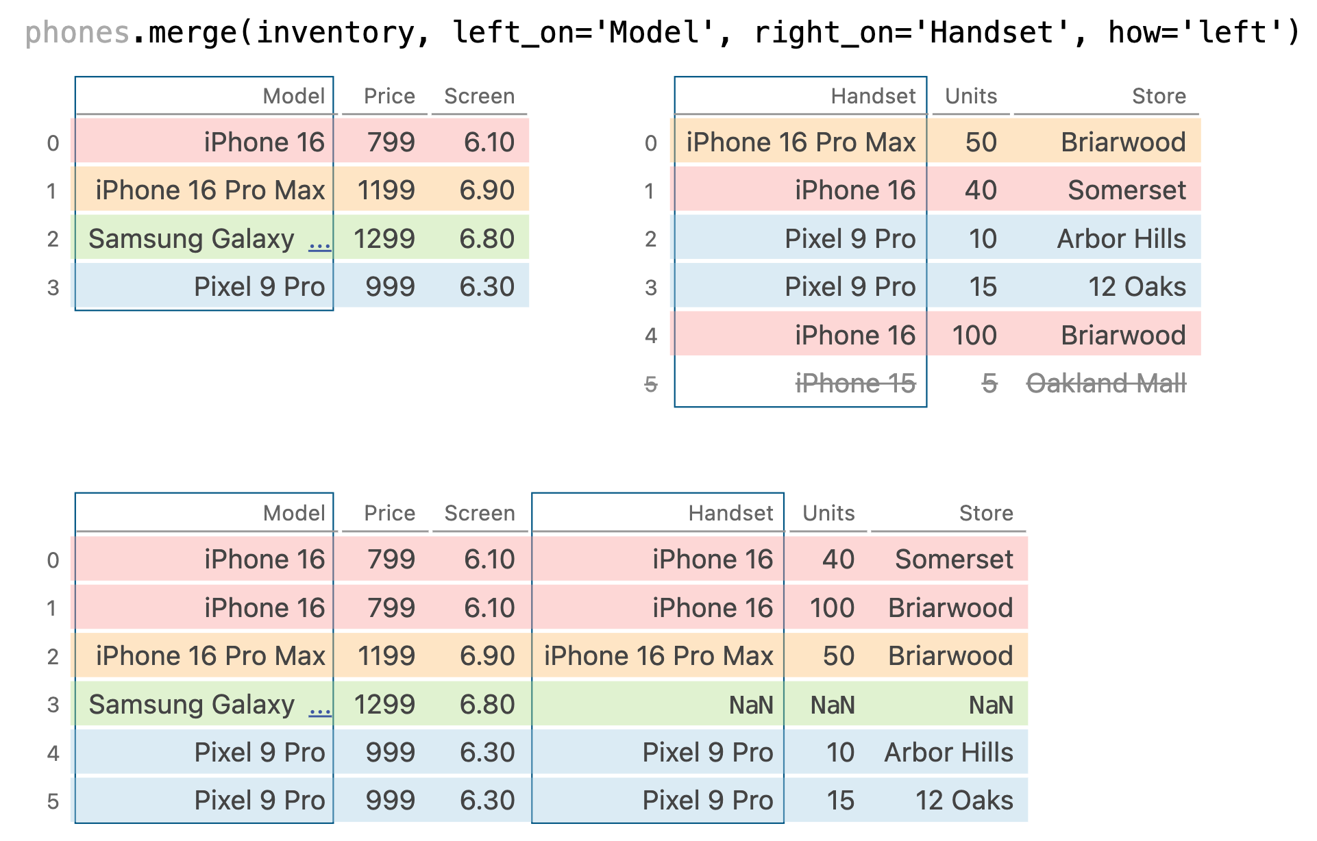
- We can change the type of join performed by changing the
howargument inmerge.
phones.merge(inventory, left_on='Model', right_on='Handset', how='left')
| Model | Price | Screen | Handset | Units | Store | |
|---|---|---|---|---|---|---|
| 0 | iPhone 16 | 799 | 6.1 | iPhone 16 | 40.0 | Somerset |
| 1 | iPhone 16 | 799 | 6.1 | iPhone 16 | 100.0 | Briarwood |
| 2 | iPhone 16 Pro Max | 1199 | 6.9 | iPhone 16 Pro Max | 50.0 | Briarwood |
| 3 | Samsung Galaxy S24 Ultra | 1299 | 6.8 | NaN | NaN | NaN |
| 4 | Pixel 9 Pro | 999 | 6.3 | Pixel 9 Pro | 10.0 | Arbor Hills |
| 5 | Pixel 9 Pro | 999 | 6.3 | Pixel 9 Pro | 15.0 | 12 Oaks |
phones.merge(inventory, left_on='Model', right_on='Handset', how='right')
| Model | Price | Screen | Handset | Units | Store | |
|---|---|---|---|---|---|---|
| 0 | iPhone 16 Pro Max | 1199.0 | 6.9 | iPhone 16 Pro Max | 50 | Briarwood |
| 1 | iPhone 16 | 799.0 | 6.1 | iPhone 16 | 40 | Somerset |
| 2 | Pixel 9 Pro | 999.0 | 6.3 | Pixel 9 Pro | 10 | Arbor Hills |
| 3 | Pixel 9 Pro | 999.0 | 6.3 | Pixel 9 Pro | 15 | 12 Oaks |
| 4 | iPhone 16 | 799.0 | 6.1 | iPhone 16 | 100 | Briarwood |
| 5 | NaN | NaN | NaN | iPhone 15 | 5 | Oakland Mall |
phones.merge(inventory, left_on='Model', right_on='Handset', how='outer')
| Model | Price | Screen | Handset | Units | Store | |
|---|---|---|---|---|---|---|
| 0 | iPhone 16 | 799.0 | 6.1 | iPhone 16 | 40.0 | Somerset |
| 1 | iPhone 16 | 799.0 | 6.1 | iPhone 16 | 100.0 | Briarwood |
| 2 | iPhone 16 Pro Max | 1199.0 | 6.9 | iPhone 16 Pro Max | 50.0 | Briarwood |
| 3 | Samsung Galaxy S24 Ultra | 1299.0 | 6.8 | NaN | NaN | NaN |
| 4 | Pixel 9 Pro | 999.0 | 6.3 | Pixel 9 Pro | 10.0 | Arbor Hills |
| 5 | Pixel 9 Pro | 999.0 | 6.3 | Pixel 9 Pro | 15.0 | 12 Oaks |
| 6 | NaN | NaN | NaN | iPhone 15 | 5.0 | Oakland Mall |
- The website pandastutor.com can help visualize DataFrame operations like these. Here's a direct link to this specific example.
Different join types handle mismatches differently
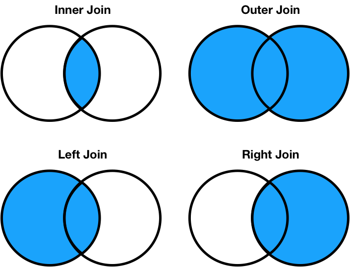
- Inner join: Keep only the matching keys (intersection).
- Outer join: Keep all keys in both DataFrames (union).
- Left join: Keep all keys in the left DataFrame, whether or not they are in the right DataFrame.
- Right join: Keep all keys in the right DataFrame, whether or not they are in the left DataFrame.
Note thata.merge(b, how='left')contains the same information asb.merge(a, how='right'), just in a different order.
mergeis flexible – you can merge using a combination of columns, or the index of the DataFrame.
- If the two DataFrames have the same column names,
pandaswill add_xand_yto the duplicated column names to avoid having columns with the same name (change these thesuffixesargument).
- There is, in fact, a
joinmethod, but it's actually a wrapper aroundmergewith fewer options.
- As always, the documentation is your friend!
pandaswill almost always try to match up index values using an outer join.
- It won't tell you that it's doing an outer join, it'll just throw
NaNs in your result!
df1 = pd.DataFrame({'a': [1, 2, 3]}, index=['hello', 'eecs398', 'students'])
df2 = pd.DataFrame({'b': [10, 20, 30]}, index=['eecs398', 'is', 'awesome'])
dfs_side_by_side(df1, df2)
| a | |
|---|---|
| hello | 1 |
| eecs398 | 2 |
| students | 3 |
| b | |
|---|---|
| eecs398 | 10 |
| is | 20 |
| awesome | 30 |
df1['a'] + df2['b']
awesome      NaN
eecs398     12.0
hello        NaN
is           NaN
students     NaN
dtype: float64
Activity setup
midwest_cities = pd.DataFrame().assign(
    city=['Ann Arbor', 'Detroit', 'Chicago', 'East Lansing'],
    state=['Michigan', 'Michigan', 'Illinois', 'Michigan'],
    today_high_temp=['79', '83', '87', '87']
)
schools = pd.DataFrame().assign(
    name=['University of Michigan', 'University of Chicago', 'Wayne State University', 'Johns Hopkins University', 'UC San Diego', 'Concordia U-Ann Arbor', 'Michigan State University'],
    city=['Ann Arbor', 'Chicago', 'Detroit', 'Baltimore', 'La Jolla', 'Ann Arbor', 'East Lansing'],
    state=['Michigan', 'Illinois', 'Michigan', 'Maryland', 'California', 'Michigan', 'Michigan'],
    graduation_rate=[0.87, 0.94, 0.78, 0.92, 0.81, 0.83, 0.91]
)
Question 🤔 (Answer at practicaldsc.org/q)
Remember that you can always ask questions anonymously at the link above!
Without writing code, how many rows are in midwest_cities.merge(schools, on='city')?
dfs_side_by_side(midwest_cities, schools)
| city | state | today_high_temp | |
|---|---|---|---|
| 0 | Ann Arbor | Michigan | 79 |
| 1 | Detroit | Michigan | 83 |
| 2 | Chicago | Illinois | 87 |
| 3 | East Lansing | Michigan | 87 |
| name | city | state | graduation_rate | |
|---|---|---|---|---|
| 0 | University of Michigan | Ann Arbor | Michigan | 0.87 |
| 1 | University of Chicago | Chicago | Illinois | 0.94 |
| 2 | Wayne State University | Detroit | Michigan | 0.78 |
| 3 | Johns Hopkins University | Baltimore | Maryland | 0.92 |
| 4 | UC San Diego | La Jolla | California | 0.81 |
| 5 | Concordia U-Ann Arbor | Ann Arbor | Michigan | 0.83 |
| 6 | Michigan State University | East Lansing | Michigan | 0.91 |
# Answer: 5.
midwest_cities.merge(schools, on='city')
| city | state_x | today_high_temp | name | state_y | graduation_rate | |
|---|---|---|---|---|---|---|
| 0 | Ann Arbor | Michigan | 79 | University of Michigan | Michigan | 0.87 |
| 1 | Ann Arbor | Michigan | 79 | Concordia U-Ann Arbor | Michigan | 0.83 |
| 2 | Detroit | Michigan | 83 | Wayne State University | Michigan | 0.78 |
| 3 | Chicago | Illinois | 87 | University of Chicago | Illinois | 0.94 |
| 4 | East Lansing | Michigan | 87 | Michigan State University | Michigan | 0.91 |
Followup activity
Without writing code, how many rows are in midwest_cities.merge(schools, on='state')?
dfs_side_by_side(midwest_cities, schools)
| city | state | today_high_temp | |
|---|---|---|---|
| 0 | Ann Arbor | Michigan | 79 |
| 1 | Detroit | Michigan | 83 |
| 2 | Chicago | Illinois | 87 |
| 3 | East Lansing | Michigan | 87 |
| name | city | state | graduation_rate | |
|---|---|---|---|---|
| 0 | University of Michigan | Ann Arbor | Michigan | 0.87 |
| 1 | University of Chicago | Chicago | Illinois | 0.94 |
| 2 | Wayne State University | Detroit | Michigan | 0.78 |
| 3 | Johns Hopkins University | Baltimore | Maryland | 0.92 |
| 4 | UC San Diego | La Jolla | California | 0.81 |
| 5 | Concordia U-Ann Arbor | Ann Arbor | Michigan | 0.83 |
| 6 | Michigan State University | East Lansing | Michigan | 0.91 |
# Answer: 13.
midwest_cities.merge(schools, on='state')
| city_x | state | today_high_temp | name | city_y | graduation_rate | |
|---|---|---|---|---|---|---|
| 0 | Ann Arbor | Michigan | 79 | University of Michigan | Ann Arbor | 0.87 |
| 1 | Ann Arbor | Michigan | 79 | Wayne State University | Detroit | 0.78 |
| 2 | Ann Arbor | Michigan | 79 | Concordia U-Ann Arbor | Ann Arbor | 0.83 |
| ... | ... | ... | ... | ... | ... | ... |
| 10 | East Lansing | Michigan | 87 | Concordia U-Ann Arbor | Ann Arbor | 0.83 |
| 11 | East Lansing | Michigan | 87 | Michigan State University | East Lansing | 0.91 |
| 12 | Chicago | Illinois | 87 | University of Chicago | Chicago | 0.94 |
13 rows × 6 columns
Activity
Fill in the blank so that the last statement evaluates to True.
df = midwest_cities.merge(schools, on='state')
df.shape[0] == (____).sum()
Don't use merge (or join) in your solution!
midwest_cities['state'].value_counts()
state
Michigan    3
Illinois    1
Name: count, dtype: int64
schools['state'].value_counts()
state
Michigan      4
Illinois      1
Maryland      1
California    1
Name: count, dtype: int64
# When we multiply the above two Series,
# the product is done by matching up the index.
midwest_cities['state'].value_counts() * schools['state'].value_counts()
state
California     NaN
Illinois       1.0
Maryland       NaN
Michigan      12.0
Name: count, dtype: float64
# When we sum the resulting Series, the missing values are ignored.
# The expression below evaluates to 13, which is the answer to the previous slide's question.
(midwest_cities['state'].value_counts() * schools['state'].value_counts()).sum()
13.0
What's next?
- How do we decide which type of visualization to create?
- How do we deal with missing values?
Reference Section
Another example
The rest of the notebook contains an additional example of how merge can be used to solve larger problems. It's a good idea to walk through it as if it's an exercise. Try to fill in the missing code here, and look at the posted HTML on the course website (or lec06-filled.ipynb) for solutions.
Name categories
This New York Times article claims that certain categories of names are becoming more popular. For example:
Forbidden names like Lucifer, Lilith, Kali, and Danger.
Evangelical names like Amen, Savior, Canaan, and Creed.
Mythological names.
It also claims that baby boomer names are becoming less popular.
- Let's see if we can verify these claims using data!
Loading in the data
- Our first DataFrame,
baby, is the same as we saw earlier in the lecture. It has one row for every combination of'Name','Sex', and'Year'.
baby
| Name | Sex | Count | Year | |
|---|---|---|---|---|
| 0 | Liam | M | 20456 | 2022 |
| 1 | Noah | M | 18621 | 2022 |
| 2 | Olivia | F | 16573 | 2022 |
| ... | ... | ... | ... | ... |
| 2085155 | Wright | M | 5 | 1880 |
| 2085156 | York | M | 5 | 1880 |
| 2085157 | Zachariah | M | 5 | 1880 |
2085158 rows × 4 columns
- Our second DataFrame,
nyt, contains the New York Times' categorization of each of several names, based on the aforementioned article.
nyt = pd.read_csv('data/nyt_names.csv')
nyt
| nyt_name | category | |
|---|---|---|
| 0 | Lucifer | forbidden |
| 1 | Lilith | forbidden |
| 2 | Danger | forbidden |
| ... | ... | ... |
| 20 | Venus | celestial |
| 21 | Celestia | celestial |
| 22 | Skye | celestial |
23 rows × 2 columns
- Issue: To find the number of babies born with (for example) forbidden names each year, we need to combine information from both
babyandnyt.
- Solution:
mergethe two DataFrames!
Returning back to our original question
Your Job: Assign category_counts to a DataFrame that contains one row for every combination of 'category' in nyt and 'Year' in baby. It should have three columns: 'category', 'Year', and 'Count', where 'Count' contains the total number of babies born with that name 'category' in that 'Year'. The first few rows of the DataFrame you're meant to create are given below.
category_counts = ...
category_counts = (
    baby
    .merge(nyt, left_on='Name', right_on='nyt_name')
    .groupby(['category', 'Year'])
    ['Count']
    .sum()
    .reset_index()
)
category_counts
| category | Year | Count | |
|---|---|---|---|
| 0 | boomer | 1880 | 292 |
| 1 | boomer | 1881 | 298 |
| 2 | boomer | 1882 | 326 |
| ... | ... | ... | ... |
| 659 | mythology | 2020 | 3516 |
| 660 | mythology | 2021 | 3895 |
| 661 | mythology | 2022 | 4049 |
662 rows × 3 columns
Once you've done that, run the cell below!
# We'll talk about plotting code soon!
import plotly.express as px
fig = px.line(category_counts, x='Year', y='Count',
              facet_col='category', facet_col_wrap=3,
              facet_row_spacing=0.15,
              width=600, height=400)
fig.update_yaxes(matches=None, showticklabels=False)